Oyster lifestage carryover project growth preliminary analysis

Post detailing preliminary analysis of oyster growth data in the USDA/WSG lifestage carry over project.

Overview

In this analysis, we looked at growth of oysters in the lifestage carry over project, which is detailed in Eric’s notebook here.

In this post I detail preliminary growth analyses. For this experiment, we have pools of lifestages in different containers, represented as replicates (n=1-4 per treatment). For adults, we had individual families tracked by tag number. We did not identify or track individual oysters and do not have replicates within individual tags. Therefore, we treat tag/container as replicates within treatment and will only have limited capacity to make inferences about family effects.

Setup

Set up workspace, set options, and load required packages.

knitr::opts_chunk$set(echo = TRUE, warning = FALSE, message = FALSE)

Load libraries

library(tidyverse)
library(ggplot2)

Read in data

growth<-read_csv("lifestage_carryover/data/size/gigas-lengths.csv")

growth<-growth%>%
  rename(tag=`tag...1`)%>%
  select(tag, `life-stage`, `init-treat`, label, month, length)%>%
  rename(lifestage=`life-stage`, treatment=`init-treat`)

growth$month<-factor(growth$month, levels=c("Oct", "Nov", "Jan"))

Look at data for whole population together

Plot growth over months for each life stage and treatment

Plot as box plot

plot<-growth%>%
  
  ggplot(aes(color=treatment, x=month, y=length))+
  geom_boxplot()+
  facet_grid(~lifestage)+
  ylab("Mean Length (cm)")+
  xlab("Month")+
  scale_color_manual(values=c("darkgray", "darkred"), name="Treatment", labels=c("Control", "Treatment"))+
  theme_classic()+
  theme(
    text=element_text(size=12, color="black")
  );plot

ggsave(plot=plot, "lifestage_carryover/output/size/mean_lengths_box.png", width=7, height=4)

Plot as mean +- standard error for all.

plot2<-growth%>%
  group_by(treatment, month, lifestage)%>%
  summarise(mean=mean(length, na.rm=TRUE), se=sd(length, na.rm=TRUE)/sqrt(length(length)))%>%
  
  ggplot(aes(color=treatment, x=month, y=mean))+
  geom_point(aes(group=interaction(treatment, lifestage)), position=position_dodge(0.3), size=1)+
  geom_errorbar(aes(ymin=mean-se, ymax=mean+se), width=0, position=position_dodge(0.3), linewidth=0.75)+
  geom_line(aes(group=treatment), position=position_dodge(0.3), linewidth=1)+
  facet_grid(~lifestage)+
  ylab("Mean Length (cm)")+
  xlab("Month")+
  scale_color_manual(values=c("darkgray", "darkred"), name="Treatment", labels=c("Control", "Treatment"))+
  theme_classic()+
  theme(
    text=element_text(size=12, color="black")
  );plot2

ggsave(plot=plot2, "lifestage_carryover/output/size/mean_lengths.png", width=7, height=4)

Run model

model<-aov(length~lifestage*month*treatment, data=growth)
summary(model)

Significant lifestage and month effects. No significant treatment effects.

                            Df Sum Sq Mean Sq  F value Pr(>F)    
lifestage                    3 383973  127991 1377.056 <2e-16 ***
month                        2   9529    4765   51.264 <2e-16 ***
treatment                    1    157     157    1.686  0.194    
lifestage:month              3  15429    5143   55.335 <2e-16 ***
lifestage:treatment          3    510     170    1.830  0.140    
month:treatment              2     15       8    0.081  0.922    
lifestage:month:treatment    3     26       9    0.094  0.963    
Residuals                 1006  93503      93   

Run plot and model by tag

Calculate mean size at each month for each replicate and calculate % growth (change/original).

replicates<-growth%>%
  group_by(treatment, month, lifestage, tag)%>%
  summarise(mean=mean(length, na.rm=TRUE))%>%
  pivot_wider(names_from=month, values_from=mean)%>%
  mutate(perc_growth_Nov=((Nov-Oct)/Oct)*100)%>%
  mutate(perc_growth_Jan=((Jan-Oct)/Oct)*100)

Plot growth for adult animals sampled in November

plot3<-replicates%>%
  select(treatment, lifestage, tag, perc_growth_Nov)%>%
  drop_na()%>%
  droplevels()%>%
  
  ggplot(aes(color=treatment, x=treatment, y=perc_growth_Nov, shape=tag))+
  geom_line(aes(group=tag), color="black")+
  geom_point(aes(group=interaction(treatment, lifestage)), position=position_dodge(0.3), size=5)+
  ylab("% growth")+
  xlab("Treatment")+
  scale_color_manual(values=c("darkgray", "darkred"), name="Treatment", labels=c("Control", "Treatment"))+
  scale_shape_manual(name="Family", values=c(15, 16, 17, 18))+
  ggtitle("Adults: Oct-Nov Growth")+
  theme_classic()+
  theme(
    text=element_text(size=12, color="black")
  );plot3

ggsave(plot=plot3, "lifestage_carryover/output/size/adults_Nov_percent_growth.png", width=4, height=4)

Test for effect of treatment.

model<-replicates%>%
  select(treatment, lifestage, tag, perc_growth_Nov)%>%
  drop_na()%>%
  droplevels()%>%
  
  aov(perc_growth_Nov~treatment, data=.)

summary(model)

Effect of treatment just barely not significant (P=0.088).

            Df Sum Sq Mean Sq F value Pr(>F)  
treatment    1  8.358   8.358   4.132 0.0883 .
Residuals    6 12.137   2.023    

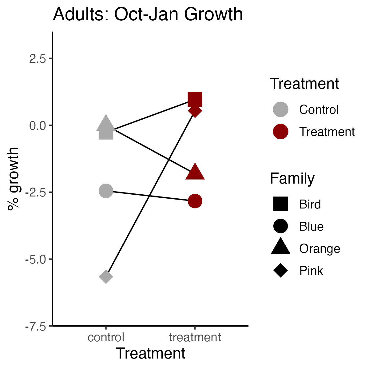
Plot growth for animals measured in January

Adults

plot4<-replicates%>%
  select(treatment, lifestage, tag, perc_growth_Jan)%>%
  filter(lifestage=="adult")%>%
  drop_na()%>%
  droplevels()%>%
  
  ggplot(aes(color=treatment, x=treatment, y=perc_growth_Jan, shape=tag))+
  geom_line(aes(group=tag), color="black")+
  geom_point(aes(group=interaction(treatment, lifestage)), position=position_dodge(0.3), size=5)+
  ylab("% growth")+
  xlab("Treatment")+
  scale_color_manual(values=c("darkgray", "darkred"), name="Treatment", labels=c("Control", "Treatment"))+
  ylim(-7, 3)+
  scale_shape_manual(name="Family", values=c(15, 16, 17, 18))+
  ggtitle("Adults: Oct-Jan Growth")+
  theme_classic()+
  theme(
    text=element_text(size=12, color="black")
  );plot4

ggsave(plot=plot4, "lifestage_carryover/output/size/adults_Jan_percent_growth.png", width=4, height=4)

Juveniles

plot5<-replicates%>%
  select(treatment, lifestage, tag, perc_growth_Jan)%>%
  filter(lifestage=="juvenile")%>%
  drop_na()%>%
  droplevels()%>%
  
  ggplot(aes(color=treatment, x=treatment, y=perc_growth_Jan, shape=tag))+
  geom_point(aes(group=interaction(treatment, lifestage)), position=position_dodge(0.3), size=5)+
  ylab("% growth")+
  xlab("Treatment")+
  scale_color_manual(values=c("darkgray", "darkred"), name="Treatment", labels=c("Control", "Treatment"))+
  scale_shape_manual(name="Replicate", values=c(15, 16, 17, 18))+
  ggtitle("Juvenile: Oct-Jan Growth")+
  theme_classic()+
  ylim(0,20)+
  theme(
    text=element_text(size=12, color="black")
  );plot5

ggsave(plot=plot5, "lifestage_carryover/output/size/juvenile_Jan_percent_growth.png", width=4, height=4)

Seed

plot6<-replicates%>%
  select(treatment, lifestage, tag, perc_growth_Jan)%>%
  filter(lifestage=="seed")%>%
  drop_na()%>%
  droplevels()%>%
  
  ggplot(aes(color=treatment, x=treatment, y=perc_growth_Jan, shape=tag))+
  #geom_line(aes(group=tag), color="black")+
  geom_point(aes(group=interaction(treatment, lifestage)), position=position_dodge(0.3), size=5)+
  ylab("% growth")+
  xlab("Treatment")+
  scale_color_manual(values=c("darkgray", "darkred"), name="Treatment", labels=c("Control", "Treatment"))+
  scale_shape_manual(name="Replicate", values=c(15, 16, 17, 18))+
  ggtitle("Seed: Oct-Jan Growth")+
  theme_classic()+
  ylim(0,250)+
  theme(
    text=element_text(size=12, color="black")
  );plot6

ggsave(plot=plot6, "lifestage_carryover/output/size/seed_Jan_percent_growth.png", width=4, height=4)

Spat

plot7<-replicates%>%
  select(treatment, lifestage, tag, perc_growth_Jan)%>%
  filter(lifestage=="spat")%>%
  drop_na()%>%
  droplevels()%>%
  
  ggplot(aes(color=treatment, x=treatment, y=perc_growth_Jan, shape=tag))+
  #geom_line(aes(group=tag), color="black")+
  geom_point(aes(group=interaction(treatment, lifestage)), position=position_dodge(0.3), size=5)+
  ylab("% growth")+
  xlab("Treatment")+
  scale_color_manual(values=c("darkgray", "darkred"), name="Treatment", labels=c("Control", "Treatment"))+
  scale_shape_manual(name="Replicate", values=c(15, 16, 17, 18))+
  ggtitle("Spat: Oct-Jan Growth")+
  theme_classic()+
  ylim(0,150)+
  theme(
    text=element_text(size=12, color="black")
  );plot7

ggsave(plot=plot7, "lifestage_carryover/output/size/spat_Jan_percent_growth.png", width=4, height=4)

Test for effect of treatment by lifestage

January all stages

model<-replicates%>%
  select(treatment, lifestage, tag, perc_growth_Jan)%>%
  drop_na()%>%
  droplevels()%>%
  
  aov(perc_growth_Jan~treatment*lifestage, data=.)

summary(model)

Effect of lifestage, no treatment effects.

                    Df Sum Sq Mean Sq F value   Pr(>F)    
treatment            1      1       1   0.015    0.904    
lifestage            3  96056   32019 325.275 3.54e-13 ***
treatment:lifestage  3    363     121   1.231    0.335    
Residuals           14   1378      98   

Interpretations

There are a few key take aways here:

Adults (1/2 of families) that were sampled in November were measured for growth in November. These families tended to be larger, so that is why lengths of adults are higher in November. All other adults and other lifestages were measured in January.
The amount of growth is much higher on a percent basis in seed and spat than adults and juveniles. This demonstrates lifestage specific investment in growth and could be interesting to explore further.
There are no strong treatment effects. There are some trends for family specific treatment effects in adults, but because we do not have replicates we cannot make any conclusions on adult family effects.

Written on February 14, 2024