This post details alignment of TagSeq sequences from the Mcap2020 developmental time series project to the symbiont genome. We will evaluate the results of this alignment to see if we have enough sequences to analyze symbiont-specific gene expression.

Dataset overview

In this project, we have gene expression, metabolomic, and physiological data across 10 developmental time points in the coral Montipora capitata in Hawaii from summer 2020.

For more information on this project, see the notebook posts for this project here.

In this analysis, I am aligning our trimmed TagSeq sequence reads to a concatenated Cladocopium-Durusdinum symbiont genome. This is becuase M. capitata hosts a mix of these genera which are detailed in this post here.

Align sequences to symbiont genome and generate gene count matrix

Sequences were trimmed and cleaned in a previous analysis as detailed in the QC section of this bioinformatics script on URI’s high performance computing cluster, Andromeda.

The full script for bioinformatics described here can be found on GitHub.

These cleaned reads were then aligned to a concatenated symbiont genome using HISAT2.

#!/bin/bash
#SBATCH -t 120:00:00
#SBATCH --nodes=1 --ntasks-per-node=20
#SBATCH --mem=100GB
#SBATCH --export=NONE
#SBATCH --output="symbiontalign_out.%j"
#SBATCH --error="symbiontalign_err.%j"

# load modules needed
module load HISAT2/2.2.1-foss-2019b
module load SAMtools/1.9-foss-2018b

#unzip reference genome
#gunzip symbiont_genome_cat.fasta.gz
#gunzip symbiont.gff.gz

# index the reference genome for Montipora capitata output index to working directory
hisat2-build -f symbiont_genome_cat.fasta ./symbiont_ref # called the reference genome (scaffolds)
echo "Referece genome indexed. Starting alingment" $(date)

# This script exports alignments as bam files
# sorts the bam file because Stringtie takes a sorted file for input (--dta)
# removes the sam file because it is no longer needed
array=($(ls clean*)) # call the clean sequences - make an array to align
for i in ${array[@]}; do
        sample_name=`echo $i| awk -F [.] '{print $2}'`
	hisat2 -p 8 --dta -x symbiont_ref -U ${i} -S ${sample_name}.sam
        samtools sort -@ 8 -o ${sample_name}.bam ${sample_name}.sam
    		echo "${i} bam-ified!"
        rm ${sample_name}.sam
done

I then used StringTie2 to compute gene abundances.

#!/bin/bash
#SBATCH -t 120:00:00
#SBATCH --nodes=1 --ntasks-per-node=20
#SBATCH --mem=100GB
#SBATCH --export=NONE
#SBATCH --output="stringtie_out.%j"
#SBATCH --error="stringtie_err.%j"

#load packages
module load StringTie/2.1.4-GCC-9.3.0

#Transcript assembly: StringTie

array=($(ls *.bam)) #Make an array of sequences to assemble
 
for i in ${array[@]}; do #Running with the -e option to compare output to exclude novel genes. Also output a file with the gene abundances
        sample_name=`echo $i| awk -F [_] '{print $1"_"$2"_"$3}'`
	stringtie -p 8 -e -B -G symbiont.gff -A ${sample_name}.gene_abund.tab -o ${sample_name}.gtf ${i}
        echo "StringTie assembly for seq file ${i}" $(date)
done
echo "StringTie assembly COMPLETE, starting assembly analysis" $(date)

Finally, I generated a gene count matrix using Prep DE.

#!/bin/bash
#SBATCH -t 120:00:00
#SBATCH --nodes=1 --ntasks-per-node=20
#SBATCH --mem=100GB
#SBATCH --export=NONE
#SBATCH --output="prepDE_out.%j"
#SBATCH --error="prepDE_err.%j"

#load packages
module load Python/2.7.15-foss-2018b #Python
module load StringTie/2.1.4-GCC-9.3.0

#Transcript assembly: StringTie
module load GffCompare/0.12.1-GCCcore-8.3.0

#Transcript assembly QC: GFFCompare

#make gtf_list.txt file
ls *.gtf > gtf_list.txt

stringtie --merge -p 8 -G symbiont.gff -o symbiont_merged.gtf gtf_list.txt #Merge GTFs to form $
echo "Stringtie merge complete" $(date)

gffcompare -r symbiont.gff -G -o merged symbiont_merged.gtf #Compute the accuracy and pre$
echo "GFFcompare complete, Starting gene count matrix assembly..." $(date)

#make gtf list text file
for filename in AH*.gtf; do echo $filename $PWD/$filename; done > listGTF.txt

python ../scripts/prepDE.py -g symbiont_gene_count_matrix.csv -i listGTF.txt #Compile the gene count matrix
echo "Gene count matrix compiled." $(date)

During the HISAT2 alignment step, alignment of reads to the symbiont genome was <4% in all samples. This indicates that we have low mapping of reads to the symbiont genome, which could be due to either low gene expression and/or symbiont abundance, or insufficient extraction of symbiont RNA. The extraction method used was optimized for the coral host, so it was not our primary target to extract symbiont RNA.

Analyze gene count matrix

With this gene count matrix, I ran an exploratory analysis using R scripts that can be found on GitHub modified from analysis of coral host gene expression.

Filtering

First, I filtered our data based on gene counts. There were 102,507 genes in the concatenated genome (total number of genes in both genomes). After removing those that were not in our dataset (row sums = 0), there were 3,489 genes in our gene count matrix. We would expect a lower number of genes expressed than present in the genome because symbionts in symbiosis with the host are in only one life stage cycle.

PoverA specfies the minimum count for a proportion of samples for each gene. Here, we are using a pOverA of 0.07. This is because we have 38 samples with a minimum of n=3 samples per lifestage. Therefore, we will accept genes that are present in 3/38 = 0.07 of the samples because we expect different expression by life stage. We are further setting the minimum count of genes to 5, such that 7% of the samples must have a gene count of >5 in order for the gene to remain in the data set.

After PoverA filtering, we have 1,218 genes in our data set. Kenkel & Matz 2017 also looked at symbiont gene expression using TagSeq data. They found ~1,700 genes in their study in the symbiont and >7,000 in the host. They did not do any additional steps in RNA extraction to specifically target the symbiont. In this study they used a PoverA of (10, 0.9) and looked at adult samples.

Visualing differences by lifestage

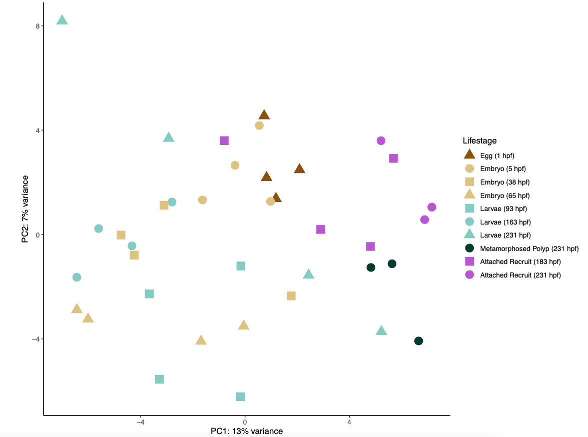
I then ran a PCA on the gene count matrix to visualize differences by life stage.

A PCA plot of gene expression shows a lot of overlap and a high degree of similarity between lifestage groups.

WGCNA

I then conducted a weighted gene coexpression network analysis (WGCNA) to look at patterns of expression correlated with life stage. This analysis detected 8 modules (soft power = 9; minimum module size=20; method by dynamic tree cut) after merging at 85% similarity.

The WGCNA heatmap looks like this:

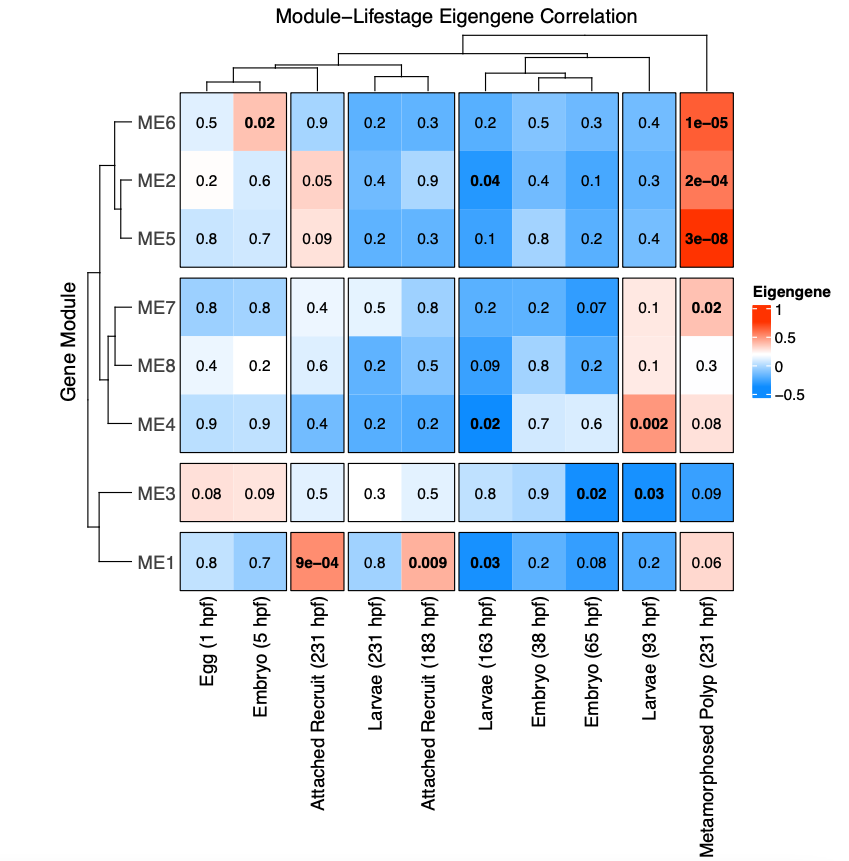
This shows modules of genes positively (red) and negatively (blue) correlated with each life stage.

There are several modules positively correlated the metamorphosed polyp group. In the PCA above, these samples group to the lower right of the points, but overlap with other lifestages.

The number of genes from each module is shown below.

Kenkel & Matz 2017 also did a WGCNA and there is a similar range of the number of genes in each module (100-400).

Eigengene values

I then visualized the variance stabilization transformed expression of genes in each module across life stages.

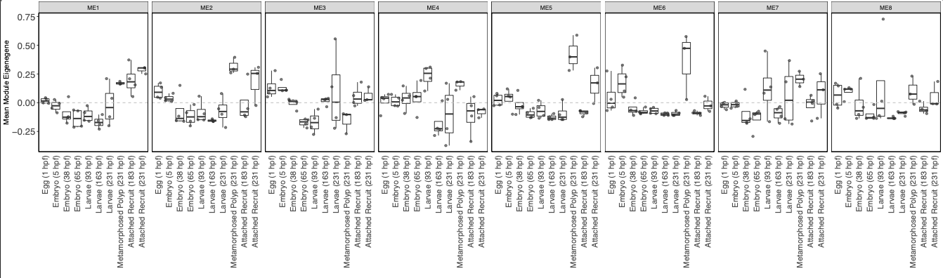
Tihs plot shows that there are a few modules with higher expression in metamorphosed polyps as seen in the WGCNA heatmap above. Gene expression patterns are not particularly distinct between lifestages.

Overall, this exploratory analysis shows that there may be variation in symbiont gene expression by life stage and in future studies we could look at analyzing gene expression in the symbiont.