This post details multivariate physiological plasticity analysis for the E5 Rules of Life project.

All code used in this post can be found in the E5 GitHub repository.

Overview

The E5 physiological time series project includes data on coral and symbiont physiology in colonies of Acropora, Pocillopora, and Porites corals in Moorea, French Polynesia. Samples of individual colonies were collected at four timepoints in the year of 2020: Jan, Mar, Sep, and Nov.

For the physiological responses collected (e.g., biomass, symbiont density, calcification, protein, antioxidant capacity), we have analyzed to investigate the influence of species, site, and time on physiology. We have found that physiological response of corals is influenced by environmental variability both across space (site) and seasons (time point).

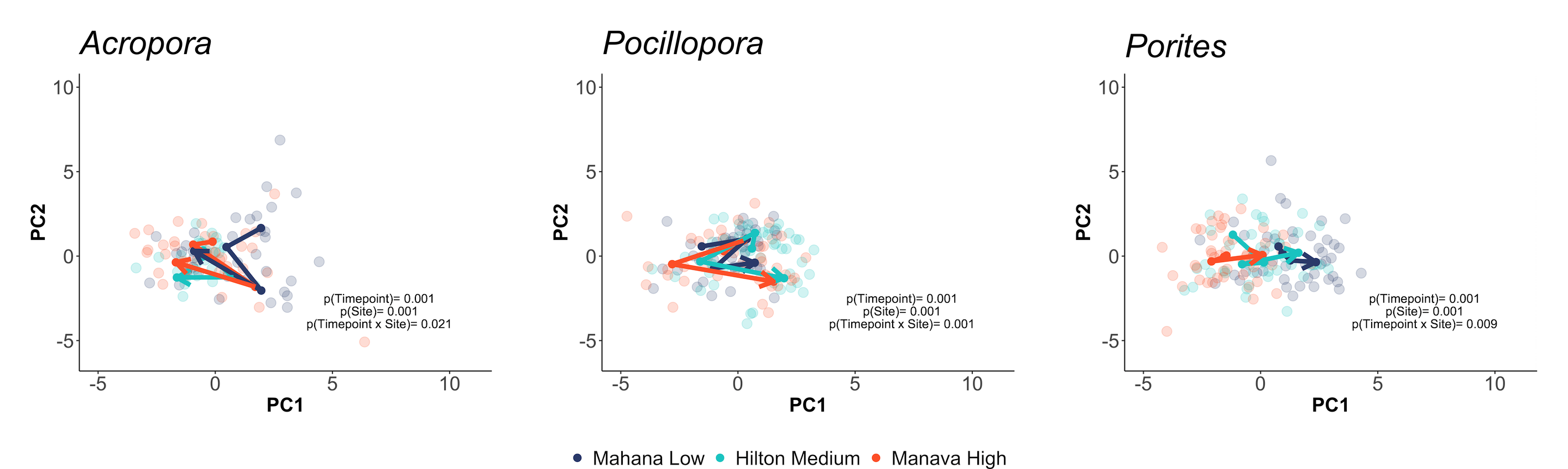
This can be visualized using trajectory principle component analyses, which visually show the movement in physiological trajectories of each species across space and time.

First, we viewed physiological responses in all responses measured:

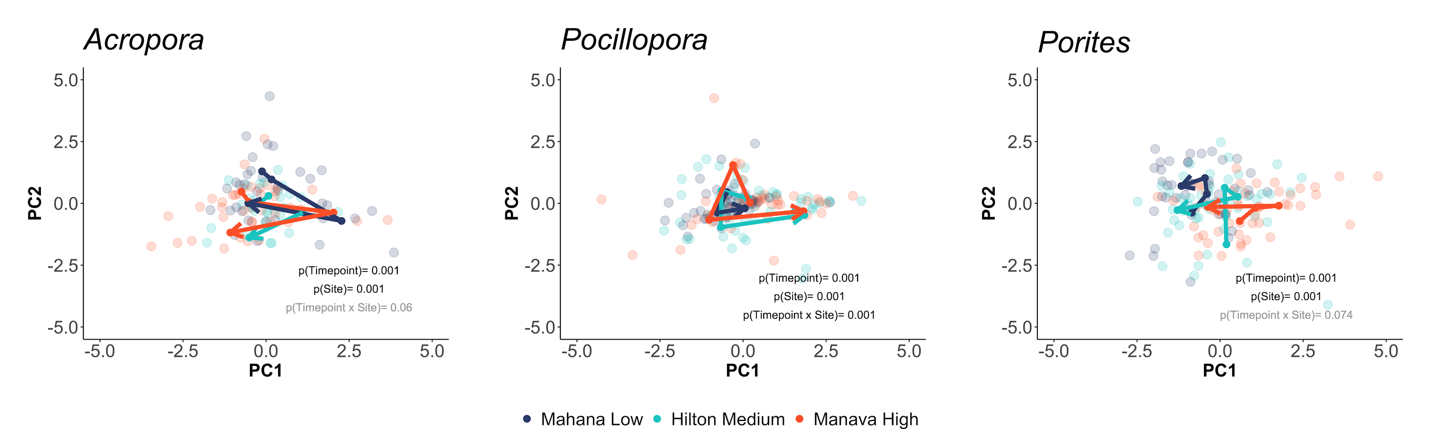
We also viewed responses separated by holobiont (e.g., calcification, host protein) responses:

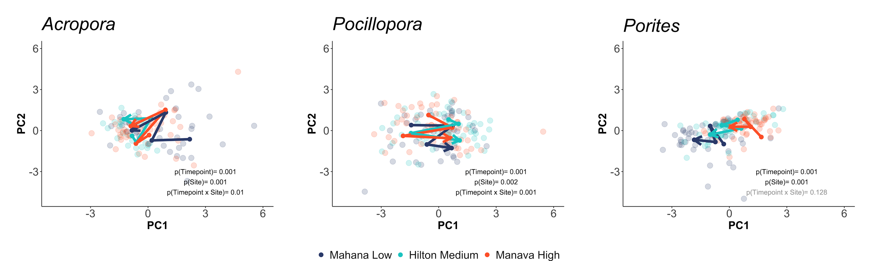
… and and symbiont responses (e.g., symbiont density, chlorophyll):

This analysis shows us that physiology varies across species, space, and time and we have additionally explored univariate drivers of these shifts. We can also see that patterns of physiological response to environmental variability differs between the host and symbiont partner.

The next step in our analysis is to quantify the “movement” or physiological acclimatization in corals between species and sites. To do this, we need to conduct an analysis to quantify the differences in physiological profiles for each colony across time in multivariate space. This post detials our analysis to do this and quanify physiological plasticity.

Analysis

This analysis utilizes Euclidean distance in multivariate physiological profiles for each colony across time. In brief, we calculate the Euclidean distance between the PCA coordinates (using all PC’s) for each colony between Jan - Mar, Jan - Sept, and Jan - Nov. These PCA coordinates are generated from the PCA analyses shown above.

The scripts to generate these calculations is as follows. This script example calculates plasticity for all responses and we repeate this for holobiont and symbiont responses.

• Load in dataframe of physiological data and use dplyr to format for our use.

master<-read.csv("Output/master_timeseries.csv")

data_all<-master%>%
  select(colony_id_corr, timepoint, species, site_code, Host_AFDW.mg.cm2, Sym_AFDW.mg.cm2, Ratio_AFDW.mg.cm2, prot_mg.mgafdw, cells.mgAFDW, cre.umol.mgafdw, Am, AQY, Rd, calc.umol.mgAFDW.hr, Total_Chl, Total_Chl_cell)%>%
  filter(Host_AFDW.mg.cm2>0)%>%
  filter(Sym_AFDW.mg.cm2>0)%>%
  filter(Ratio_AFDW.mg.cm2>0)%>%
  filter(Sym_AFDW.mg.cm2<20)%>%
  filter(prot_mg.mgafdw<1.5)%>% #remove outliers
  rename(Host_Biomass=Host_AFDW.mg.cm2, Symbiont_Biomass=Sym_AFDW.mg.cm2, S_H_Biomass_Ratio=Ratio_AFDW.mg.cm2, Host_Protein=prot_mg.mgafdw, Symbiont_Density=cells.mgAFDW, Antiox_Capacity=cre.umol.mgafdw, Calc=calc.umol.mgAFDW.hr)

This data frame has colony, timepoint, species, and site identifiers in rows with physiological parameters for each in columns.

• Generate a PCA in the vegan package by keeping only complete cases and scaling and centering the data. We also generate a data frame that has the identifiers for each row.

data_all<-data_all[complete.cases(data_all), ]

scaled_all<-prcomp(data_all[c(5:16)], scale=TRUE, center=TRUE) 

all_info<-data_all[c(1:4)]

• We then obtain a file that has the multivariate coordinates for each sample. The data frame has sample information in rows and the coordinate for each PC in columns.

all_data<-scaled_all%>%
  augment(all_info)%>%
  group_by(timepoint, site_code, species, colony_id_corr)%>%
  mutate(code=paste(timepoint, colony_id_corr))

all_data<-as.data.frame(all_data)

row.names(all_data)<-all_data$code

all_data<-all_data[6:17]
head(all_data)

The data frame looks like this:

                    .fittedPC1  .fittedPC2  .fittedPC3   .fittedPC4  .fittedPC5   .fittedPC6   .fittedPC7    .fittedPC8   .fittedPC9  .fittedPC10   .fittedPC11
timepoint1 ACR-139 -1.092554899  1.31118246 -0.18831065  1.019204635 -0.10989941 -0.031524089  0.173102427 -0.0324509521  0.043750699 -0.326213307  0.1740722665
timepoint1 ACR-140 -0.925392751  1.61558439 -0.68659720  0.651995985  0.58748251 -0.378884073 -0.472616145  0.2670025481  0.120231724 -0.122747789 -0.0329355853
timepoint1 ACR-145 -1.830410343  1.56047048 -1.46958427  1.404187366 -0.44726904  0.478756040  0.163938348 -0.9461384136  0.101712379  0.664160494 -0.1158255179
timepoint1 ACR-150  0.823393665  2.80399813 -0.76410146  1.821100061 -0.98939827 -0.599291849 -0.033438311  1.1796691659 -0.099541109  0.365550525  0.1046269188
timepoint1 ACR-165 -1.194331027 -0.07814978 -1.12799853  0.859084096 -0.57676311 -0.403215120 -0.355485784 -0.6249028929 -0.191247642  0.131296174 -0.0992637370

• Next, use the dist() function to calculate euclidian distances between each sample’s multivariate coordinates obtained above.

dist_all<-dist(all_data, diag = FALSE, upper = FALSE, method="euclidean")

dist_all <- melt(as.matrix(dist_all), varnames = c("row", "col"))

This produces a data frame with the distance values and looks like this. This data frame shows the colony that the comparison is calculated for and the timepoints that the distance is calculated between. Value contains the Euclidean distance.

Timepoint1 Timepoint2 Colony1    value
1 timepoint1 timepoint2 ACR-140 1.209748
2 timepoint1 timepoint2 ACR-150 3.615525
3 timepoint1 timepoint2 ACR-173 3.231441
4 timepoint1 timepoint2 ACR-186 2.197203
5 timepoint1 timepoint2 ACR-225 1.750085
6 timepoint1 timepoint2 ACR-229 6.018570

• We then tidy the dataset to provide columns that will help us select only the comparisons we want to make. Here, we want to keep only comparisons within colony (i.e., how much did one colony change between time points) and we want to keep only comparisons between time point 1 (Jan) and each subsequent timepoint, keeping Jan as our reference value.

dist_all<-dist_all%>%
  separate(row, into=c("Timepoint1", "Colony1"), sep=" ")%>%
  separate(col, into=c("Timepoint2", "Colony2"), sep=" ")%>%
  filter(value>0.0)%>% #remove distances between the same points
  mutate(condition=if_else(Colony1==Colony2, "TRUE", "FALSE"))%>%
  filter(condition=="TRUE")%>% #keep within colony comparisons
  filter(Timepoint1=="timepoint1")%>% #only keep comparisons that are relative to TP1
  select(Timepoint1, Timepoint2, Colony1, value)

#add in timepoint column
dist_all_mean<-dist_all%>%
  mutate(timepoint=paste(Timepoint1, "-", Timepoint2))

#add in metadata
dist_all_mean$site_code<-all_info$site_code[match(dist_all_mean$Colony1, all_info$colony_id_corr)]
dist_all_mean$species<-all_info$species[match(dist_all_mean$Colony1, all_info$colony_id_corr)]

• We then generate a figure that displays the mean colony plasticity (AKA mean Euclidean distance value) and view by site and species.

dist_all_plot2<-dist_all_mean%>%
  group_by(species, site_code)%>%
  summarise(mean=mean(value), sd=sd(value), N=length(value), se=sd/sqrt(N))%>% #calculate means at group level
  
    ggplot(aes(x = site_code, y = mean, fill=species, group=interaction(species, site_code))) +
    geom_line(aes(group=species, color=species), position=position_dodge(0.15), size=2)+
    geom_point(pch = 21, size=5, position = position_dodge(0.15)) + 
    geom_errorbar(aes(ymin=mean-se, ymax=mean+se, group=interaction(species, site_code)), width=0, color="black", position=position_dodge(0.15))+
    scale_fill_manual(name="Species", values = c("darkgray", "orange", "purple"))+
    scale_color_manual(name="Species", values = c("darkgray", "orange", "purple"))+
    xlab("Site") + 
    ylab(expression(bold("Colony-Specific Euclidean Distance")))+
    geom_text(x=2, y=0.7, size=4, label="Site p<0.001", color="black")+
    geom_text(x=2, y=0.4, size=4, label="Species p<0.001", color="black")+
    geom_text(x=2, y=0.1, size=4, label="Interaction p=0.040", color="black")+
    theme_classic() + 
    ylim(0,7)+
    ggtitle("A. All Responses")+
    theme(
      legend.position="right",
      legend.title=element_text(face="bold", size=14),
      legend.text=element_text(size=14, face="italic"),
      axis.title=element_text(face="bold", size=14),
      axis.text=element_text(size=14, color="black"), 
      strip.text.x=element_text(face="italic", size=14),
      title=element_text(face="bold", size=16)
      ); dist_all_plot2

• The output is seen in the Results section below. Finally, we run an ANOVA to test for differences between species and site in plasticity scores.

dist_all_model<-aov(value~site_code*species, data=dist_all_mean)
summary(dist_all_model)`

Outputs of these results are shown in the figures below.

This process is then repeated for physiological profiles for 1) all response; 2) holobiont responses, and 3) symbiont responses.

Results

The results of this analysis look like this:

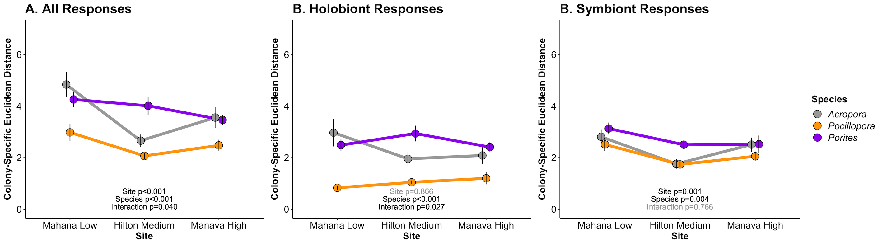
There are a few interesting preliminary conclusions from these results.

1. Pocillopora has lower plasticity, which is driven by reduced plasticity in the host/holobiont as compared to the symbiont.
2. Porites and Acropora have higher plasticity, but Acropora has reduced plasticity at the Hilton site, where it is not naturally found.
3. Plasticity is variable by site, indicating environmental influence on physiological plasticity.
4. Species plasticity is determined by site (species x site effects) for all responses and holobiont responses, but this interaction is not influential at the symbiont level. Instead, symbiont plasticity is higher in Porites and has a small decrease across sites, particularly in the Hilton site.
5. Holobiont and symbiont physiological plasticity respond differently across site and species.

Next Steps

The next steps are to develop environmental indices for the seasonal time points to place time effects into the context of temperature and light. We will continue further analyzing this data and consider modeling how plasticity correlates or relates to metrics of performance such as calcification.