


DESeq LRT and Functional Enrichment Analysis of Mcap2020 TagSeq Data
This post details analysis of the Montipora capitata TagSeq data set using a DESeq2 likelihood ratio test approach and subsequent functional enrichment using goseq. I previously found an error in my functional enrichment code that is corrected in this revised analysis.
Below I have included code and figures generated.
Overview of approach
In this study, I sampled early life stages of Montipora capitata coralsacross a developmental time series spanning fertilized eggs (1 hour post fertilization, hpf) to attached recruits (255 hpf). This sampling was from wildtype gametes collected in Kaneohe Bay, Hawaii in collaboration with the Coral Resilience Lab at the Hawaii Institute of Marine Biology. I then used TagSeq sequencing to investigate gene expression across this time series, with sequencing of samples from 1 hpf to 231 hpf including eggs, embryos, larvae, metamorphosed polyps (metamorphosed polyps not yet fully attached to the substrate), and attached recruits (attachment to substrate after metamorphosis).
The GitHub repository for this project can be found here and all notebook post regarding this project are here.
This post details analysis of TagSeq gene count matrix usin a DESeq2 workflow. I have previously analyzed this data using a WGCNA approach, but have revised this to a likelihood ratio test (LRT) method in DESeq2. This has provided a statistically robust way to analyze this data with a method that is more appropriate for the data structure and questions of interest.
In this study, I also collected physiological data, metabolomics, ITS2 sequencing, and respirometry data. See the GitHub repository, my notebook, and a previous preprint for more information.
In my previous analyses, I found that I was incorrectly specifying the GO term list that went into the functional enrichment analysis. This has been corrected in this script below.

In this TagSeq dataset, each developmental stage is identified by the stage and hours post fertilization (hpf). There are n=4 replicates per life stage. There are no random effects to account for.
This analysis uses the reference genome for Montipora capitata available at Cyanophora - Version 3. See the publication detailing this annotation here.
Code and Results
The script for this analysis is on GitHub here.
This analyses uses the DESeq2 package in R - see the vingette for more detailed information on this package here.
My hypotheses are:
- Gene expression will vary significantly between lifestages.
- There will be genes that are differentially expressed across the time series of development characterizing developmental phases.
Load required libraries
library("tidyverse")
library("genefilter")
library("DESeq2")
library("RColorBrewer")
library("WGCNA")
library("flashClust")
library("gridExtra")
library("ComplexHeatmap")
library("goseq")
library("dplyr")
library("clusterProfiler")
library("pheatmap")
library("magrittr")
library("rtracklayer")
library("GenomicRanges")
library("plyranges")
library("GSEABase")
library("stats")
library("ggdendro")
library("GO.db")
library("rrvgo")
library("DESeq2")
library("genefilter")
library("factoextra")
library("vegan")
library("EnhancedVolcano")
library("VennDetail")
library("viridis")
library("cowplot")
library("DEGreport")
library("circlize")
library("tibble")
Data input and filtering
Import the data files. Data files include a sample metadata with lifestage information for each sample and the gene count matrix produced using this code and detailed in my notebook here.
#load metadata sheet with sample name and developmental stage information
metadata <- read.csv("Mcap2020/Data/TagSeq/Sample_Info.csv", header = TRUE, sep = ",")
head(metadata)

#load gene count matrix generated from cluster computation
gcount <- as.data.frame(read.csv("Mcap2020/Output/TagSeq/Mcapitata_gene_count_matrix_V3.csv", row.names="gene_id"), colClasses = double)
head(gcount)

#remove metamorphosed recruit 1 because this was the timepoint that we only had one sample for: D36, AH23
#gcount<-gcount[ , !(names(gcount) %in% c("AH23"))]
gcount<-gcount[ , !(names(gcount) %in% c("AH23_S54_L002.gtf"))]

metadata <- metadata%>%
  filter(!sample_id=="AH23")
Remove genes with 0 counts across all samples (genes not detected).
nrow(gcount)
gcount<-gcount %>%
     mutate(Total = rowSums(.[, 1:38]))%>%
    filter(!Total==0)%>%
    dplyr::select(!Total)
nrow(gcount)
There are 54,384 genes in the reference genome and included in the gene count matrix. This was filtered down to 34,223 by removing genes with row sums of 0 (those not detected in our data).
Next, conduct filtering using pOverA.
pOverA: Specifying the minimum count for a proportion of samples for each gene. Here, we are using a pOverA of 0.07. This is because we have 38 samples with a minimum of n=3 samples per lifestage (n=3 for one stage, the others are n=4). Therefore, we will accept genes that are present in 3/38 = 0.07 of the samples because we expect different expression by life stage. We are further setting the minimum count of genes to 10, such that 7% of the samples must have a gene count of >10 in order for the gene to remain in the data set.
Filter in the package genefilter. Pre-filtering our dataset improves quality of statistical analysis by removing low-coverage counts and will also reduce the memory size dataframe and increase the speed of the transformation and testing functions.
filt <- filterfun(pOverA(0.07,10))

#create filter for the counts data
gfilt <- genefilter(gcount, filt)

#identify genes to keep by count filter
gkeep <- gcount[gfilt,]

#identify genes to keep by count filter
gkeep <- gcount[gfilt,]

#identify gene lists
gn.keep <- rownames(gkeep)

#gene count data filtered in PoverA, P percent of the samples have counts over A
gcount_filt <- as.data.frame(gcount[which(rownames(gcount) %in% gn.keep),])

#How many rows do we have before and after filtering?
nrow(gcount) #Before
nrow(gcount_filt) #After
Before filtering, we had 34,223 genes. After filtering for pOverA, we have 11,475 genes. This indicates that there were many genes present in <7% of samples at <10 counts per gene, indicating low expression.
In order for the DESeq2 algorithms to work, the SampleIDs on the metadta file and count matrices have to match exactly and in the same order. The following R chunk will check to make sure that these match.
#Checking that all row and column names match. Should return "TRUE"
all(rownames(metadata$sample_id) %in% colnames(gcount_filt))
all(rownames(metadata$sample_id) == colnames(gcount_filt))
Match metadata sample id’s.
result<-sub("_.*", "", colnames(gcount_filt)) #keep characters before _
#result2<-sub(".*AH", "", result) #keep characters after X
colnames(gcount_filt)<-result #keep just sample number
Display current order of metadata and gene count matrix.
metadata$sample_id
colnames(gcount_filt)
Order metadata the same as the column order in the gene matrix.
list<-colnames(gcount_filt)
list<-as.factor(list)

metadata$sample_id<-as.factor(metadata$sample_id)

# Re-order the levels
metadata$sample_id <- factor(as.character(metadata$sample_id), levels=list)
# Re-order the data.frame
metadata_ordered <- metadata[order(metadata$sample_id),]
metadata_ordered$sample_id

metadata_ordered<-metadata_ordered%>%
  dplyr::select(sample_id, lifestage, hpf, code)
Reorder the lifestage factor. Reorder to be in developmental order:
- Eggs (1 hpf)
- Embryos (5 hpf)
- Embryos (38 hpf)
- Embryos (65 hpf)
- Larvae (93 hpf)
- Larvae (163 hpf)
- Larvae (231 hpf)
- Metamorphosed polyp (231 hpf)
- Attached recruit (183 hpf)
- Attached recruit (231 hpf)
This sets the fertilized egg (1 hpf) as the reference level.
head(metadata_ordered)
levels(as.factor(metadata_ordered$lifestage))

metadata_ordered$lifestage<-as.factor(metadata_ordered$lifestage)

metadata_ordered$lifestage<-fct_relevel(metadata_ordered$lifestage, "Egg (1 hpf)", "Embryo (5 hpf)", "Embryo (38 hpf)", "Embryo (65 hpf)", "Larvae (93 hpf)", "Larvae (163 hpf)", "Larvae (231 hpf)", "Metamorphosed Polyp (231 hpf)", "Attached Recruit (183 hpf)", "Attached Recruit (231 hpf)")

levels(as.factor(metadata_ordered$lifestage))

#output metadata for other analyses
#write_csv(metadata_ordered, "Mcap2020/Data/TagSeq/metadata_ordered.csv")
We are now ready to construct a DESeq2 model.
Construct DESeq2 data set
Create a DESeqDataSet design from the gene count matrix and lifestage categories. Here, we set the design to look at lifestage to test for any differences in gene expression across timepoints.
#Set DESeq2 design
gdds <- DESeqDataSetFromMatrix(countData = gcount_filt,
                              colData = metadata_ordered,
                              design = ~lifestage)
First we are going to log-transform the data using a variance stabilizing transforamtion (VST). This function calculates a variance stabilizing transformation (VST) from the fitted dispersion-mean relation(s) and then transforms the count data (normalized by division by the size factors or normalization factors), yielding a matrix of values which are now approximately homoskedastic (having constant variance along the range of mean values).
To do this we first need to calculate the size factors of our samples. This is a rough estimate of how many reads each sample contains compared to the others. In order to use VST (the faster log2 transforming process) to log-transform our data, the size factors need to be less than 4.
Chunk should return TRUE if <4.
SF.gdds <- estimateSizeFactors(gdds) #estimate size factors to determine if we can use vst  to transform our data. Size factors should be less than 4 for us to use vst
print(sizeFactors(SF.gdds)) #View size factors

all(sizeFactors(SF.gdds)) < 4
All size factors are less than 4, so we can use a VST transformation. blind=FALSE should be used for transforming data for downstream analysis, where the full use of the design information should be made. blind=FALSE will skip re-estimation of the dispersion trend, if this has already been calculated. If many of genes have large differences in counts due to the experimental design, it is important to set blind=FALSE for downstream analysis.
gvst <- vst(gdds, blind=FALSE) #apply a variance stabilizing transformation to minimize effects of small counts and normalize wrt library size
head(assay(gvst), 3) #view transformed gene count data for the first three genes in the dataset.
Conduct PERMANOVA for all genes
Export vst normalized gene counts for PERMANOVA test.
test<-t(assay(gvst)) #export as matrix
test<-as.data.frame(test)

#add category columns
test$Sample<-rownames(test)
test$Lifestage<-metadata$lifestage[match(test$Sample, metadata$sample_id)]
Build PERMANOVA model for all genes that passed filtering by lifestage.
scaled_test <-prcomp(test[c(1:11475)], scale=TRUE, center=TRUE)
fviz_eig(scaled_test)

# scale data
vegan <- scale(test[c(1:11475)])

# PerMANOVA
permanova<-adonis2(vegan ~ Lifestage, data = test, method='eu')
permanova
40% variance was explained on PC1, with 10% or less by remaining PCs.
Gene expression is significantly different between lifestages (p=0.001).
Permutation test for adonis under reduced model
Terms added sequentially (first to last)
Permutation: free
Number of permutations: 999

adonis2(formula = vegan ~ Lifestage, data = test, method = "eu")
          Df SumOfSqs      R2      F Pr(>F)
Lifestage  9   318674 0.75057 9.3618  0.001 ***
Residual  28   105901 0.24943
Total     37   424575 1.00000
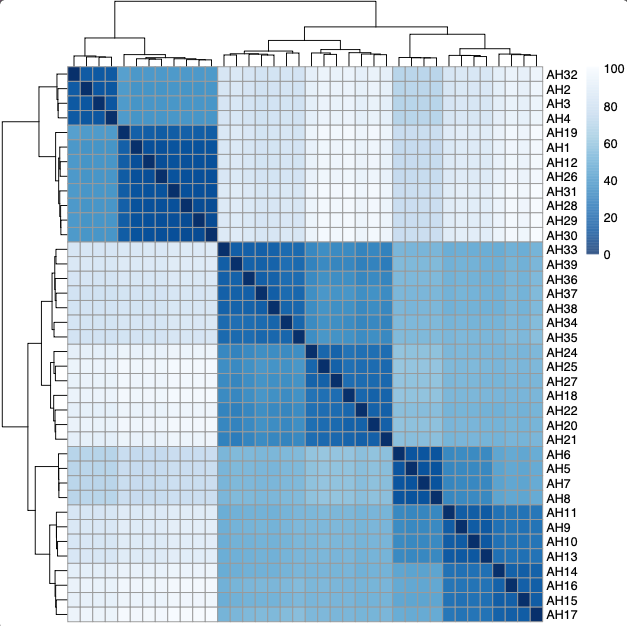
Next, plot a PCA and heatmap of sample to sample distances for all genes.
Plot a heatmap to sample to sample distances
gsampleDists <- dist(t(assay(gvst))) #calculate distance matix
gsampleDistMatrix <- as.matrix(gsampleDists) #distance matrix
rownames(gsampleDistMatrix) <- colnames(gvst) #assign row names
colnames(gsampleDistMatrix) <- NULL #assign col names
colors <- colorRampPalette( rev(brewer.pal(9, "Blues")) )(255) #assign colors

save_pheatmap_pdf <- function(x, filename, width=7, height=7) {
   stopifnot(!missing(x))
   stopifnot(!missing(filename))
   pdf(filename, width=width, height=height)
   grid::grid.newpage()
   grid::grid.draw(x$gtable)
   dev.off()
}

pht<-pheatmap(gsampleDistMatrix, #plot matrix
         clustering_distance_rows=gsampleDists, #cluster rows
         clustering_distance_cols=gsampleDists, #cluster columns
         col=colors) #set colors

#save_pheatmap_pdf(pht, "Mcap2020/Figures/TagSeq/GenomeV3/pheatmap.pdf")
Generate a PCA of gene expression for all genes.
gPCAdata <- plotPCA(gvst, intgroup = c("lifestage"), returnData=TRUE, ntop=11475) #use ntop to specify all genes
percentVar <- round(100*attr(gPCAdata, "percentVar")) #plot PCA of samples with all data

levels(gPCAdata$lifestage)

allgenesfilt_PCA_visual <-
  ggplot(data=gPCAdata, aes(PC1, PC2, shape=lifestage, colour=lifestage)) +
  geom_point(size=5, stroke=1) +
  xlab(paste0("PC1: ",percentVar[1],"% variance")) +
  ylab(paste0("PC2: ",percentVar[2],"% variance")) +

  scale_shape_manual(name="Lifestage", values = c("Egg (1 hpf)"=1, "Embryo (5 hpf)"=2, "Embryo (38 hpf)"=3, "Embryo (65 hpf)"=4, "Larvae (93 hpf)"=5, "Larvae (163 hpf)"=6, "Larvae (231 hpf)"=8, "Metamorphosed Polyp (231 hpf)"=11, "Attached Recruit (183 hpf)"=10, "Attached Recruit (231 hpf)"=12)) +

  scale_colour_manual(name="Lifestage", values = c("Egg (1 hpf)"="#8C510A", "Embryo (5 hpf)"="#DFC27D", "Embryo (38 hpf)"="#DFC27D", "Embryo (65 hpf)"="#DFC27D", "Larvae (93 hpf)"="#80CDC1", "Larvae (163 hpf)"="#80CDC1", "Larvae (231 hpf)"="#80CDC1", "Metamorphosed Polyp (231 hpf)"="#003C30", "Attached Recruit (183 hpf)"="#BA55D3", "Attached Recruit (231 hpf)"="#BA55D3")) +
  #xlim(-40,40)+
  #ylim(-40,40)+
  #coord_fixed()+
  theme_classic() + #Set background color
  theme(panel.border = element_rect(colour = "black", fill=NA), # Set border
                     #panel.grid.major = element_blank(), #Set major gridlines
                     #panel.grid.minor = element_blank(), #Set minor gridlines
                     axis.line = element_line(colour = "black"), #Set axes color
        plot.background=element_blank(),
        axis.title=element_text(size=14),
        axis.text=element_text(size=12, color="black"))  + #Set the plot background
  theme(legend.position = ("right"))
allgenesfilt_PCA_visual

ggsave("Mcap2020/Figures/TagSeq/GenomeV3/DESeq/PCA_all_genes.pdf", allgenesfilt_PCA_visual, width=8, height=5)

Global gene expression changes across lifestages. This is expected because early life stages are going through extensive physiological changes that require shifts in molecular function.
There are three developmental phases that are apparent from the PCA plots.
- Early development (1 hpf - 38 hpf)
- Mid development (65 hpf - 163 hpf)
- Late development (183 hpf - 231 hpf)
We will later use these groupings for functional enrichment analyses.
Run DESeq Results Tests
There are two statistical tests we can use in DESeq2: Wald test and likelihood ratio test (LRT). Here is what I have learned about each and why I chose the method that I use below.
Here is the information from the DESeq2 vingette: “DESeq2 offers two kinds of hypothesis tests: the Wald test, where we use the estimated standard error of a log2 fold change to test if it is equal to zero, and the likelihood ratio test (LRT). The LRT examines two models for the counts, a full model with a certain number of terms and a reduced model, in which some of the terms of the full model are removed. The test determines if the increased likelihood of the data using the extra terms in the full model is more than expected if those extra terms are truly zero. The LRT is therefore useful for testing multiple terms at once, for example testing 3 or more levels of a factor at once, or all interactions between two variables. The LRT for count data is conceptually similar to an analysis of variance (ANOVA) calculation in linear regression, except that in the case of the Negative Binomial GLM, we use an analysis of deviance (ANODEV), where the deviance captures the difference in likelihood between a full and a reduced model.”
Given this information, the Wald test is most appropriate for cases where there are comparisons between 2 groups or when you are interested in conducting pairwise comparisons between 2 or more groups. The LRT test is appropriate for cases where there are multiple levels of a factor where you are interested in the whole effect of that factor (e.g., a time series where you want to detect any effects across time).
Because we have multiple levels in a time series, and I am interested in genes that change across time, I will use the LRT test.
We will select DEG’s that have a p-value adjusted < 0.05 (we have a lot of DEG’s, so I am chosing a more stringent cut off). The p-value is the only statistic associated with the LRT statistical test, so filtering by fold change is not appropriate here. I will keep all genes at p-value adjusted < 0.05 at any fold change. As I ran this test, I found that we had a very high number of DEG’s and I increased the stringency of the p-value adjusted to keep highly significant genes at p<0.001 (detailed below).
Run test using the LRT to look for genes that change significantly across the time series. There is only one main effect (lifestage), so the reduced model is just the intercept.
DEG <- DESeq(gdds, test="LRT", reduced=~1)
From this, we are going to filter by adjusted p value <0.05, this is generated by the LRT test statistic. We had 9180 DEGs at P<0.05. I also ran at P<0.01 because we need a higher threshold due to the high number of DEGs. This was only reduced to 8686 with P<0.01. It was reduced further to P<0.001 with 8127 genes. 88.5% of genes were retained in the dataset at a stringent threshold. I chose this stringent threshold to streamline analyses and keep only the most strongly significant genes as the most conservative approach.
DEG_results<-results(DEG)
DEG_results <- as.data.frame(subset(DEG_results, padj<0.001))

DEG_results$gene <- rownames(DEG_results)
rownames(DEG_results) <- NULL
There are 8127 DEGs out of 11,475 total genes (70.8% of all genes are DEGs). Most genes are differentially expressed across time. This is expected for a developmental time series spanning eggs to recruits due to the drastic changes in function.
Subset our gene count matrix to keep only DEGs and conduct VST transformation as done above.
DEG_results_vst <- gdds[unique(DEG_results$gene)]
dim(DEG_results_vst)

DEG_results_vst <- varianceStabilizingTransformation(DEG_results_vst)
Plot heatmap of DEGs
Next, plot a heat map of the identified DEGs from the LRT test.
Set themes and metadata.
legend_names_col = colnames(assay(DEG_results_vst))

df <- as.data.frame(colData(gdds)[,c("lifestage")])
names(df)<-"lifestage"
rownames(df) <- legend_names_col

levels(df$lifestage)

df$lifestage <- factor(as.character(df$lifestage))

ann_colors = list(
    lifestage = c("Egg (1 hpf)"="#8C510A", "Embryo (5 hpf)"="tan2", "Embryo (38 hpf)"="tan3",  "Embryo (65 hpf)"="tan", "Larvae (93 hpf)"="#80CDC1", "Larvae (163 hpf)"="cyan2", "Larvae (231 hpf)"="cyan", "Metamorphosed Polyp (231 hpf)"="#003C30", "Attached Recruit (183 hpf)"="#BA55D3", "Attached Recruit (231 hpf)"="pink3")
)
Plot heatmap on scaled (z-scores) of vst normalized gene counts.
dev.off()
pdf("Mcap2020/Figures/TagSeq/GenomeV3/DESeq/DEG_heatmap_development.pdf", width=10, height=10)
pheatmap(assay(DEG_results_vst), cluster_rows=TRUE, show_rownames=FALSE, color=inferno(10), show_colnames=FALSE, fontsize_row=3, scale="row", cluster_cols=TRUE, annotation_col=df, annotation_colors = ann_colors, labels_col=legend_names_col, clustering_distance_rows = "euclidean", clustering_distance_cols = "euclidean", cutree_rows = 3)
dev.off()
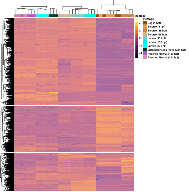
Eggs through 38 hpf group together; 65-163 hpf group together, attached recruits group together, and larvae and polyps at 231 hpf group together as expected from our PCA plot.
PERMANOVA and PCA of DEGs
Conduct PERMANOVA by lifestage for DEGs.
Export data for PERMANOVA test.
test_DEG<-t(assay(DEG_results_vst)) #export as matrix
test_DEG<-as.data.frame(test_DEG)

#add category columns
test_DEG$sample<-rownames(test_DEG)
test_DEG$lifestage<-metadata$lifestage[match(test_DEG$sample, metadata$sample)]
Build PERMANOVA model for DEG’s that are different between lifestages for the 8,127 DEGs.
dim(test_DEG)

scaled_test_DEG <-prcomp(test_DEG[c(1:8127)], scale=TRUE, center=TRUE)
fviz_eig(scaled_test_DEG)

# scale data
vegan_DEG <- scale(test_DEG[c(1:8127)])

# PerMANOVA
permanova_DEG<-adonis2(vegan_DEG ~ lifestage, data = test_DEG, method='eu')
permanova_DEG
62% of variance is explained on PC1 (separating early from mid/late phases) with 14% explained on PC2 (separating early/mid and late phases).
Permutation test for adonis under reduced model
Terms added sequentially (first to last)
Permutation: free
Number of permutations: 999

adonis2(formula = vegan_DEG ~ lifestage, data = test_DEG, method = "eu")
          Df SumOfSqs     R2      F Pr(>F)
lifestage  9   250210 0.8321 15.418  0.001 ***
Residual  28    50489 0.1679
Total     37   300699 1.0000
Plot PCA.
gPCAdata_DEG <- plotPCA(DEG_results_vst, intgroup = c("lifestage"), returnData=TRUE, ntop=8127) #use ntop to specify all genes
percentVar_DEG <- round(100*attr(gPCAdata_DEG, "percentVar")) #plot PCA of samples with all data

levels(gPCAdata$lifestage)

DEG_PCA <-
  ggplot(data=gPCAdata_DEG, aes(PC1, PC2, shape=lifestage, colour=lifestage)) +
  geom_point(size=5, stroke=1) +
  xlab(paste0("PC1: ",percentVar_DEG[1],"% variance")) +
  ylab(paste0("PC2: ",percentVar_DEG[2],"% variance")) +

  scale_shape_manual(name="Lifestage", values = c("Egg (1 hpf)"=1, "Embryo (5 hpf)"=2, "Embryo (38 hpf)"=3, "Embryo (65 hpf)"=4, "Larvae (93 hpf)"=5, "Larvae (163 hpf)"=6, "Larvae (231 hpf)"=8, "Metamorphosed Polyp (231 hpf)"=11, "Attached Recruit (183 hpf)"=10, "Attached Recruit (231 hpf)"=12)) +

  scale_colour_manual(name="Lifestage", values = c("Egg (1 hpf)"="#8C510A", "Embryo (5 hpf)"="#DFC27D", "Embryo (38 hpf)"="#DFC27D", "Embryo (65 hpf)"="#DFC27D", "Larvae (93 hpf)"="#80CDC1", "Larvae (163 hpf)"="#80CDC1", "Larvae (231 hpf)"="#80CDC1", "Metamorphosed Polyp (231 hpf)"="#003C30", "Attached Recruit (183 hpf)"="#BA55D3", "Attached Recruit (231 hpf)"="#BA55D3")) +

  #coord_fixed()+
  theme_classic() + #Set background color
  theme(panel.border = element_rect(colour = "black", fill=NA), # Set border
                     #panel.grid.major = element_blank(), #Set major gridlines
                     #panel.grid.minor = element_blank(), #Set minor gridlines
                     axis.line = element_line(colour = "black"), #Set axes color
        plot.background=element_blank(),
        axis.title=element_text(size=14),
        axis.text=element_text(size=12, color="black"))  + #Set the plot background
  theme(legend.position = ("right")); DEG_PCA

ggsave("Mcap2020/Figures/TagSeq/GenomeV3/DESeq/PCA_DEG.pdf", DEG_PCA, width=8, height=5)
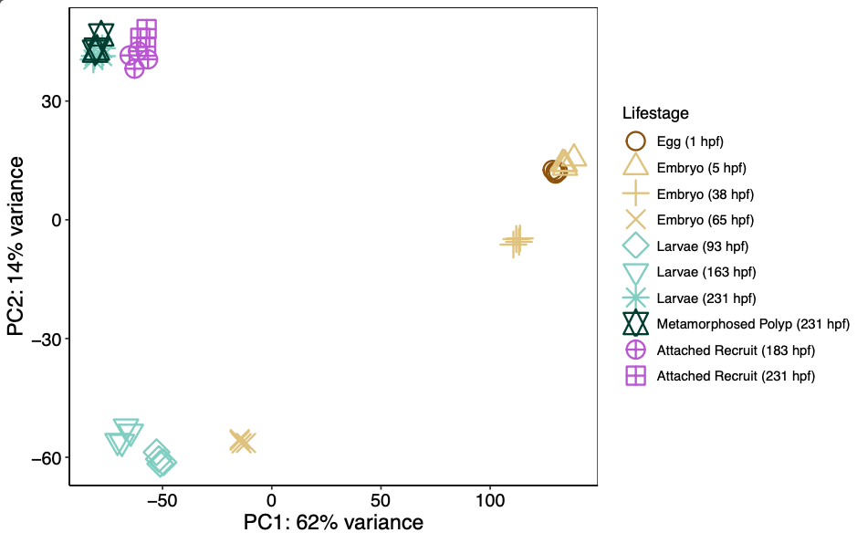
We still see the same clear three groupings for early, mid, and late developmental phases.
Save gene lists for functional enrichment
DEG_results: List of DEG’s and fold change/pvalues
DEG_results_vst: Count matrix of genes from DEG list
8,127 genes in DEG dataset
dim(DEG_results)
head(DEG_results)

deg_results_list<-DEG_results%>%
  dplyr::select(gene, everything())
write_csv(deg_results_list, "Mcap2020/Output/TagSeq/GenomeV3/DESeq/deg_list.csv")

dim(DEG_results_vst)
deg_counts<-t(assay(DEG_results_vst))
deg_counts<-as.data.frame(deg_counts)
dim(deg_counts)
deg_counts$sample<-rownames(deg_counts)
deg_counts<-deg_counts%>%
  dplyr::select(sample, everything())
write_csv(deg_counts, "Mcap2020/Output/TagSeq/GenomeV3/DESeq/deg_counts.csv")
List of all genes in the dataset (gvst) = 11,475 genes which will serve as the background set of genes for functional enrichment.
dim(gvst)
all_genes<-t(assay(gvst))
all_genes<-as.data.frame(all_genes)
dim(all_genes)
all_genes$sample<-rownames(all_genes)
all_genes<-all_genes%>%
  dplyr::select(sample, everything())

write_csv(file="Mcap2020/Output/TagSeq/GenomeV3/DESeq/all_genes.csv", all_genes)
Now that we have identified DEGs that significantly change by lifestage, we will use clustering to interpret how these change change across the developmental time series.
Detect clusters of LRT results
I am using the degPatterns function in the DEGreport package in R for this analysis. This code was adapted from a tutorial here.
This code analyzes the DEGs for temporal patterns in expression. Analogous to a WGCNA, this analysis will identify sets of genes (depending on the minimum number of genes to be included in a cluster) that share expression patterns. For example, it could identify genes that increase over time, those that decrease over time, or those that peak in one particular life stage, for example. This will allow us to interpret the DEGs in a way that is meaningful across the developmental time series.
Run a DESeq2 model and extract results as we did above.
# results
DEG <- DESeq(gdds, test="LRT", reduced=~1)

# Extract results for LRT
res_LRT <- results(DEG)

# View results for LRT
res_LRT
Filter for genes padj <0.001 as done above to identify the same 8,127 DEGs. I am repeating this process here because I can then start the script at this point if desired.
padj.cutoff <- 0.001

# Create a tibble for LRT results
res_LRT_tb <- res_LRT %>%
  data.frame() %>%
  rownames_to_column(var="gene") %>%
  as_tibble()

# Subset to return genes with padj < target
sigLRT_genes <- res_LRT_tb %>%
  dplyr::filter(padj < padj.cutoff)

# Get number of significant genes
nrow(sigLRT_genes)
There are 8127 genes that change across developmental time at p<0.001.
Prepare the dataframe as a matrix and obtain lifestage metadata for each sample. Obtain vst transformed values for DEGs.
clustering_sig_genes <- sigLRT_genes %>%
  arrange(padj) #genes in rows, stats in columns

matrix<-assay(gvst) #genes in rows, sample ID in columns

meta <- metadata_ordered %>%
  dplyr::select(sample_id, lifestage) #sample id and lifestage column

rownames(meta)<-meta$sample_id

meta<-meta%>%
  dplyr::select(lifestage) #sample ID in rows, one column of lifestage

# Obtain transformed values for those significant genes
cluster_vst <- matrix[clustering_sig_genes$gene, ] #rows are DEGs and columns are sample ID
Conduct the clustering using the degPatterns function from the ‘DEGreport’ package to view scaled (z-score) normalized gene expression across life stages.
I am going to run with a setting for a minimum of 100 genes per cluster because we have a high number of DEGs and are interested in broad scale developmental patterns. This script will identify clusters (i.e., groups of genes that share expression patterns) and keep those with 100 or more genes. Clusters will be identified with numbers (i.e., clusters 1 through 10). Not all numbers will remain present - those with fewer than the gene number threshold will be removed. For example, a set of clusters may result in Clusters 1, 2, 4, and 5 with cluster 3 removed for having too few genes.
This will take awhile to run because the number of DEGs is large. Takes about 10 minutes to run.
# Use the `degPatterns` function from the 'DEGreport' package to show gene clusters across sample groups
clusters <- degPatterns(cluster_vst, metadata = meta, time = "lifestage", col=NULL, plot=FALSE, minc = 100)
6372 genes were clustered with cluster size >100. Therefore, 1755 genes are not included in these clusters because they belong to clusters that had fewer than 100 genes included.
Plot the clusters that were identified. These plots show z-scores of VST normalized gene counts across life stages.
dev.off()
cluster_plot<-ggplot(clusters[["normalized"]],
        aes(x=lifestage, y=value)) +
  facet_wrap(~ cluster)+
   geom_point(colour="darkgray", size=1) +
  ylab("Z-score of VST normalized gene counts")+
  xlab("")+
   # change the method to make it smoother
   geom_smooth(aes(group=genes), method = "loess", colour="red", linewidth=0.1, se=FALSE)+
   geom_smooth(aes(group=1), method = "loess", colour="black")+
  geom_hline(yintercept=0, linetype="dashed")+
  geom_vline(xintercept=3, linetype="dotted")+
  geom_vline(xintercept=6, linetype="dotted")+
  theme_classic()+
  theme(
    axis.text.x = element_text(angle=90, hjust=1, vjust=1)
  );cluster_plot

ggsave(cluster_plot, filename="Mcap2020/Figures/TagSeq/GenomeV3/DESeq/cluster_plot.pdf", width=10, height=8)
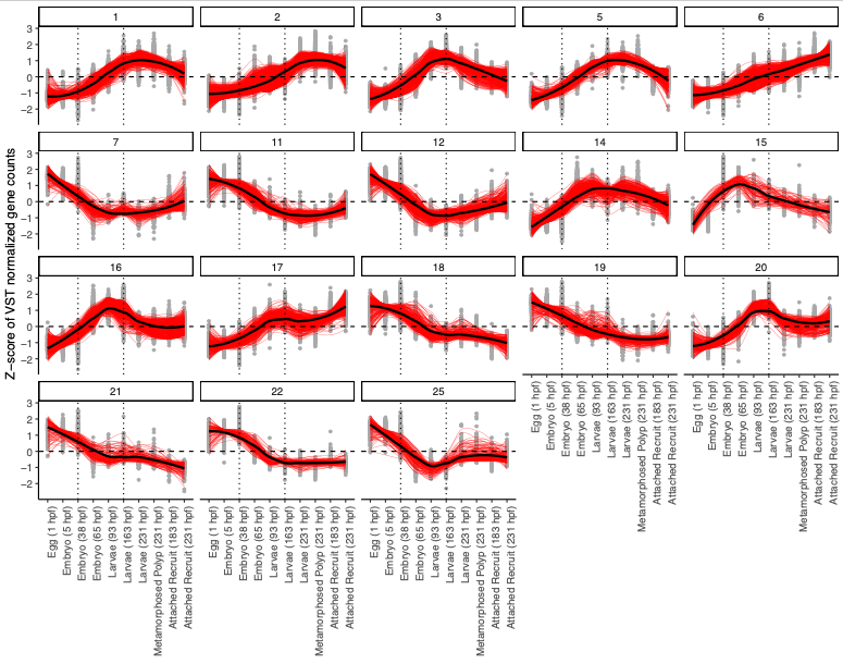
Super cool! Each cluster shows a different developmental pattern (i.e., peaking in one particular group, increasing, decreasing, etc.).
From these plots, I see that clusters group into our same three developmental patterns identified above. I added dotted lines to show the divisions in those developmental groups.
I then categorized the clusters as:
- Early development: expression peaking at or before 38 hpf - includes eggs and embryos (clusters 7, 11, 12, 18, 19, 21, 22, 25)
- Mid development: expression peaking between 65 and 163 hpf - includes late embryos and larvae (clusters 3, 14, 15, 16, 20)
- Late development: expression peaking between 183 and 231 hpf - includes latelarvae, polyps, and recruits (clusters 1, 2, 5, 6, 17)
These patterns continue to match our PCA and heatmap visualizations above.
#early development
#7, 11, 12, 18, 19, 21, 22, 25
early<-c("7", "11", "12", "18", "19", "21", "22", "25")

#mid development
#3, 14, 15, 16, 20
mid<-c("3", "14", "15", "16", "20")

#late development
#1, 2, 5, 6, 17
late<-c("1", "2", "5", "6", "17")
Plot averages of these clusters for each developmental period by grouping all clusters within each developmental pattern.
cluster_data<-clusters[["normalized"]]
cluster_data<-as.data.frame(cluster_data)
cluster_data<-cluster_data%>%
  dplyr::select(genes, merge, value, lifestage, cluster)%>%
  mutate(pattern=if_else(cluster %in% early, "Early",
                          if_else(cluster %in% mid, "Mid",
                                  if_else(cluster %in% late, "Late", NA))))

cluster_data$pattern<-factor(cluster_data$pattern, levels=c("Early", "Mid", "Late"))

cluster_plot2<-ggplot(cluster_data,
        aes(x=lifestage, y=value)) +
  facet_wrap(~ pattern)+
   geom_point(colour="darkgray", size=1) +
  ylab("Z-score of VST normalized gene counts")+
  xlab("")+
   # change the method to make it smoother
   geom_smooth(aes(group=genes), method = "loess", colour="red", linewidth=0.1, se=FALSE)+
   geom_smooth(aes(group=1), method = "loess", colour="black", linewidth=1, se=TRUE)+
  geom_hline(yintercept=0.5, linetype="dashed")+
  geom_vline(xintercept=3.5, linetype="dotted")+
  geom_vline(xintercept=6.5, linetype="dotted")+
  theme_classic()+
  theme(
    axis.text.x = element_text(angle=90, hjust=1, vjust=1)
  );cluster_plot2

ggsave(cluster_plot2, filename="Mcap2020/Figures/TagSeq/GenomeV3/DESeq/cluster_plot_patterns.pdf", width=8, height=6)
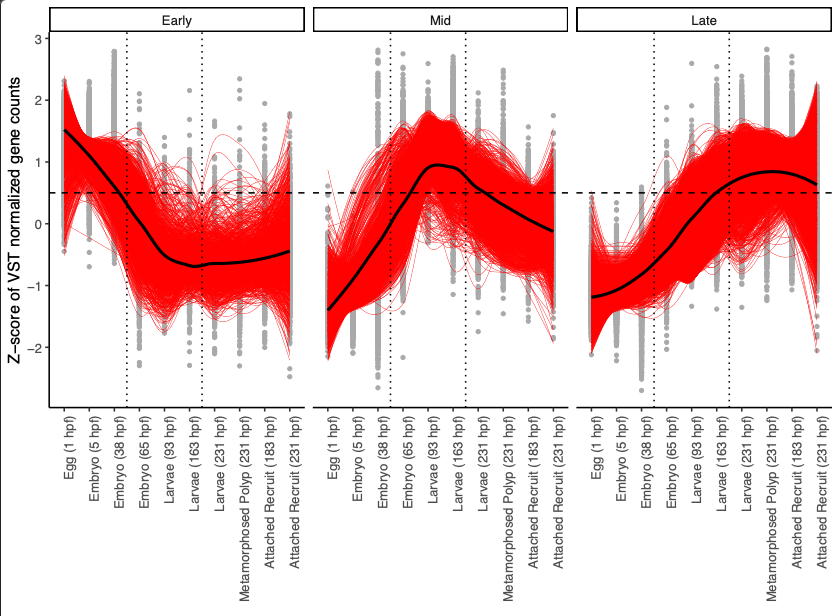
This confirms the three developmental patterns. We will conduct functional enrichment at the level of developmental pattern by concatenating the lists of genes from all modules included in each pattern.
Next, find the total number of genes in each cluster and developmental pattern.
Extract the list of genes in each cluster.
# Rename and extract information
group <- clusters$df %>%
          rename(gene=genes)
Assign developmental pattern.
group <- group%>%
  mutate(pattern=if_else(cluster %in% early, "Early",
                         if_else(cluster %in% mid, "Mid",
                                 if_else(cluster %in% late, "Late", NA))))
Display number of genes in each cluster and total genes in each developmental pattern.
ngenes<-clusters$summarise%>%
  as.data.frame()

ngenes<-ngenes%>%dplyr::select(cluster, n_genes)%>%unique()%>%mutate(pattern=if_else(cluster %in% early, "Early",
                         if_else(cluster %in% mid, "Mid",
                                 if_else(cluster %in% late, "Late", NA))))

ngenes

ngenes%>%
  group_by(pattern)%>%
  summarise(sum=sum(n_genes))
There are:
- 1845 genes in early development clusters
- 2789 genes in late development clusters
- 1696 genes in mid development clusters
Plot fold change of DEGs
deg_FC <- DEG_results %>%
  dplyr::arrange(log2FoldChange) %>%

  ggplot(aes(x=log2FoldChange, y=reorder(gene, -log2FoldChange), colour=padj)) +
  #facet_grid(~contrast, scales="free_y")+
  geom_point(size=1)+
  scale_colour_gradientn(name="P(adj)", colours = colorspace::heat_hcl(7))+
  geom_segment(aes(x=0, xend=log2FoldChange, y=gene, yend=gene),linewidth=1) +
  geom_vline(xintercept = 0, linetype = "dashed") + # Add vertical line
  theme_classic() +
  ylab("Gene")+
  theme(legend.position = "right",
        axis.text.y = element_blank(),
        axis.text.x = element_text(size=14),
        strip.text=element_text(size=16),
        axis.title.y = element_text(size=16, face="bold"),
        axis.title.x = element_text(size = 16, face = "bold"),
        plot.title = element_text(size = 18, face = "bold"))+
  ggtitle(''); deg_FC

ggsave(plot=deg_FC, "Mcap2020/Figures/TagSeq/GenomeV3/DESeq/DEG_foldchange.png", height=6, width=8)
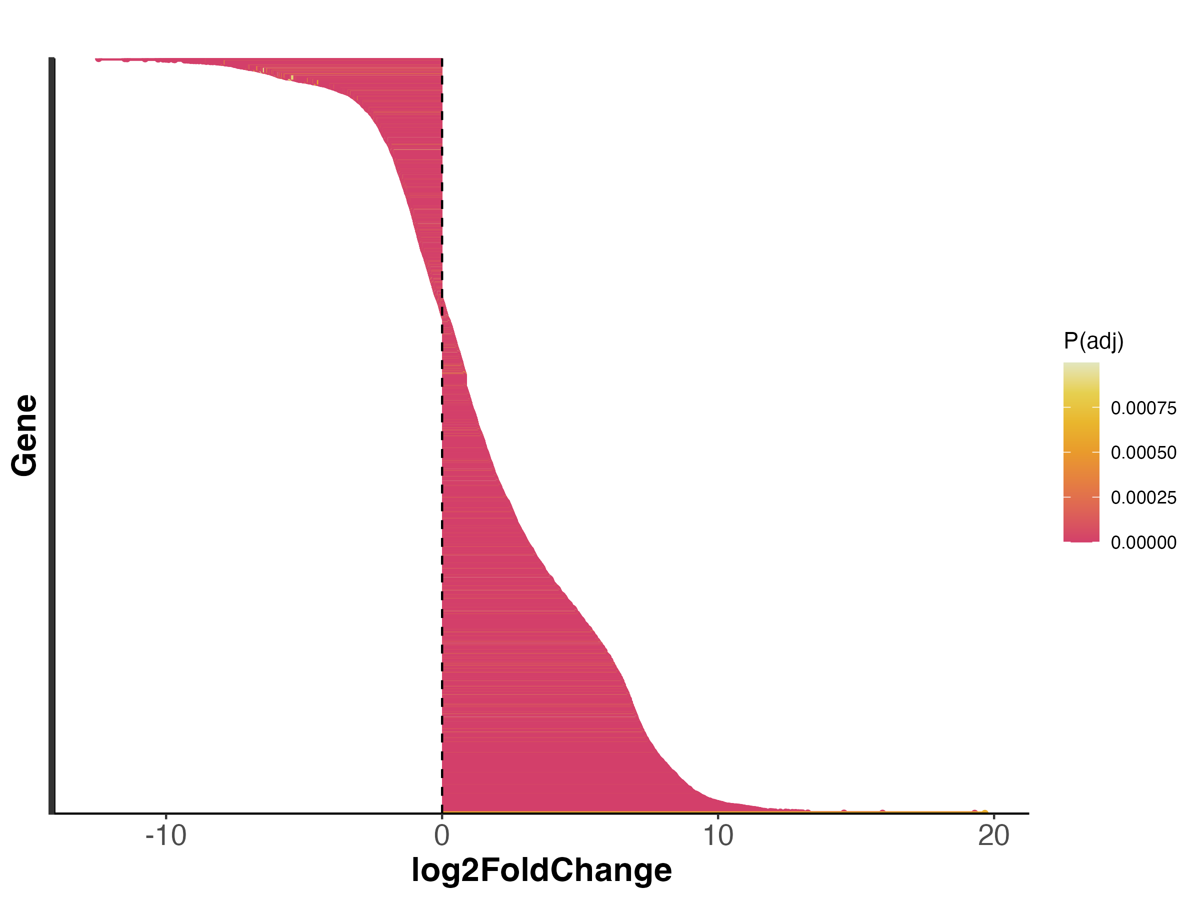
There are some genes that change a lot (log2FoldChange >10) and some that change to a lesser degree.
Functional enrichment of genes identified in clusters
Next, proceed with functional enrichment of genes in each developmental pattern using the goseq and rrvgo packages.
Read in file with a list of all genes detected that passed filtering.
all_genes<-read.csv("Mcap2020/Output/TagSeq/GenomeV3/DESeq/all_genes.csv")
Read in file of DEG’s identified through DESeq2 LRT test.
DEG_list<-read.csv("Mcap2020/Output/TagSeq/GenomeV3/DESeq/deg_list.csv")
DEG_counts<-read.csv("Mcap2020/Output/TagSeq/GenomeV3/DESeq/deg_counts.csv")
Get gene length information to allow for length bias corrections in goseq. Longer genes are more likely to be detected due to higher likelihood of amplification during library preparation.
I am using the GFF file associated with the reference genome used in this dataset available at Cyanophora - Version 3.
#import file
gff <- rtracklayer::import("Mcap2020/Data/TagSeq/Montipora_capitata_HIv3.genes.gff3") #if this doesn't work, restart R and try again

transcripts <- subset(gff, type == "transcript") #keep only transcripts

transcripts_gr <- makeGRangesFromDataFrame(transcripts, keep.extra.columns=TRUE) #extract length information

transcript_lengths <- width(transcripts_gr) #isolate length of each gene

seqnames<-transcripts_gr$ID #extract list of gene id

lengths<-cbind(seqnames, transcript_lengths)

lengths<-as.data.frame(lengths) #convert to data frame
Read in annotation file.
I downloaded the functional annotation (version 3) from: http://cyanophora.rutgers.edu/montipora/Montipora_capitata_HIv3.genes.EggNog_results.txt.gz (EggNog) and http://cyanophora.rutgers.edu/montipora/Montipora_capitata_HIv3.genes.KEGG_results.txt.gz (KEGG).
I unzipped the files on my desktop. I then removed the # in #query in the first column, otherwise it does not read in column names.
Mcap.annot <- read.table("Mcap2020/Data/TagSeq/Montipora_capitata_HIv3.genes.EggNog_results.txt",  quote="", sep="\t", header=TRUE)
dim(Mcap.annot)

# column names
head(Mcap.annot)
tail(Mcap.annot)

Mcap.annot<-Mcap.annot%>%
  rename(gene=query)

names(Mcap.annot)
This functional annotation has 24,072 genes. This is 44% of total protein predicted genes described in the publication associated with this annotation. See the publication detailing this annotation here.
Total the number of genes in our DEG list that have available annotation information.
names(Mcap.annot)

#remove sample column name
probes = names(all_genes)
#probes <- gsub("sample", "", probes)
#probes <- probes[probes != ""]

probes2annot = match(probes, Mcap.annot$gene) #match genes in datExpr to genes in annotation file, note I removed the # before query in this file before loading

# The following is the number of probes without annotation
sum(is.na(probes2annot))

row_nas<-which(is.na(probes2annot))

#view the genes that do not have a match in the annotation file
missing<-as.data.frame(probes[row_nas])
#print(missing)
There are 3,395 of our genes that were expressed that are not present in the annotation file, this is expected, not all genes will have annotation information.
Reduce annotation file to only contain genes detected in our dataset.
filtered_Mcap.annot <- Mcap.annot[Mcap.annot$gene %in% probes, ]
dim(filtered_Mcap.annot)
The annotation file now only contains genes that were detected in our dataset that have annotation information. This is 8,081 out of the 11,475 genes in our dataset.
Add in gene length to the annotation file.
filtered_Mcap.annot$length<-lengths$transcript_lengths[match(filtered_Mcap.annot$gene, lengths$seqnames)]

which(is.na(filtered_Mcap.annot$length)) #all genes have lengths
All genes have length information.
Format GO terms to remove dashes and quotes.
#remove dashes, remove quotes from columns and separate by semicolons (replace , with ;) in KEGG_ko, KEGG_pathway, and Annotation.GO.ID columns
head(filtered_Mcap.annot$GOs)
filtered_Mcap.annot$GOs <- gsub(",", ";", filtered_Mcap.annot$GOs)
filtered_Mcap.annot$GOs <- gsub('"', "", filtered_Mcap.annot$GOs)
filtered_Mcap.annot$GOs <- gsub("-", NA, filtered_Mcap.annot$GOs)
Files are now ready for functional enrichment. I first ran functional enrichment for each cluster. I will not be detailing that analysis in this post. Instead, I combined gene lists for each developmental pattern and conducted functional enrichment at the level of developmental pattern.
Conduct enrichment for developmental patterns
Merge in relevant annotation information to the DEG list file. Merge to only keep genes that were identified to belong to a cluster.
group_list<-left_join(group, filtered_Mcap.annot, by="gene")
Conduct functional enrichment using goseq and rrvgo. Our background gene set is all genes detected and that passed filtering in our gene count matrix. Our test gene set is the list of genes associated with each developmental pattern. We will filter for GO terms that are present at FDR p-value adjusted <0.05. We will also use semantic similarity to remove reduntant terms and generate parent terms for visualization. Functional enrichment was conducted at the Biological Process ontogeny.
I use loops to generate functional enrichment analyses and plots for levels of interest. Here, I’ll be running a loop to conduct analysis for each developmental pattern (“Early”, “Mid”, and “Late). This can be replaced with whatever treatment group is required.
The required files for functional enrichment are:
ALL.vector: a list of all genes as the background set (i.e., all genes detected and passed filtering)LENGTH.vector: a list of lengths for all genes as the background setID.vector: a list of DEGs to be testedGO.terms: a list of all GO terms present in the background gene setgene.vector: a vector generated from ALL.vector and ID.vector to generate a list of all genes with 1 indicating a DEG and 0 indicating that the gene is not a DEG
These files are generated in the loop below.
After generating these vectors, I conducted enrichment using goseq. First, I ran the nullp function to generate a bias vector that accounts for length bias by gene length for each gene.
pwf<-nullp(gene.vector, bias.data=LENGTH.vector)
Next, I ran goseq using the Wallenius model for Biological Process GO terms.
GO.wall<-goseq(pwf, gene2cat=GO.terms, test.cats=c("GO:BP"), method="Wallenius", use_genes_without_cat=TRUE)
This is conducted in the loop below.
pattern_list<-levels(as.factor(group_list$pattern))

for (pattern_id in pattern_list) {

    ### Generate vector with names of all genes detected in our dataset
    ALL.vector <- c(filtered_Mcap.annot$gene)

    ### Generate length vector for all genes
    LENGTH.vector <- as.integer(filtered_Mcap.annot$length)

    ### Generate vector with names in just the contrast we are analyzing
    ID.vector <- group_list%>%
      filter(pattern==pattern_id)%>%
      pull(gene)

    ##Get a list of GO Terms for all genes detected in our dataset
    GO.terms <- filtered_Mcap.annot%>%
      dplyr::select(gene, GOs)

    ##Format to have one goterm per row with gene ID repeated
    split <- strsplit(as.character(GO.terms$GOs), ";")
    split2 <- data.frame(v1 = rep.int(GO.terms$gene, sapply(split, length)), v2 = unlist(split))
    colnames(split2) <- c("gene", "GOs")
    GO.terms<-split2

    ##Construct list of genes with 1 for genes in contrast and 0 for genes not in the contrast
    gene.vector=as.integer(ALL.vector %in% ID.vector)
    names(gene.vector)<-ALL.vector#set names

    #weight gene vector by bias for length of gene
    pwf<-nullp(gene.vector, bias.data=LENGTH.vector)

    #run goseq using Wallenius method for all categories of GO terms
    GO.wall<-goseq(pwf, gene2cat=GO.terms, test.cats=c("GO:BP"), method="Wallenius", use_genes_without_cat=TRUE)

    GO <- GO.wall[order(GO.wall$over_represented_pvalue),]
    colnames(GO)[1] <- "GOterm"

    #adjust p-values
    GO$bh_adjust <-  p.adjust(GO$over_represented_pvalue, method="BH") #add adjusted p-values

    #Filtering for p < 0.05
    GO <- GO %>%
        dplyr::filter(bh_adjust<0.05) %>%
        dplyr::arrange(., ontology, bh_adjust)

    #Write file of results
    write_csv(GO, file = paste0("Mcap2020/Output/TagSeq/GenomeV3/DESeq/functional_enrichment/goseq_", pattern_id, ".csv"))

}
Verify that all files have the correct dimensions.
length(ALL.vector)
length(LENGTH.vector)
dim(pwf)
length(unique(GO.terms$gene))
length(gene.vector)
length(ID.vector)
All the dimensions of the input dataframes count to 8081, the expected number of genes (all genes in our dataset with annotation information). ID.vector should be length expected from your DEGs.
Create an empty dataframe to populate with enriched terms (only do this once).
pattern_go_results <- data.frame()
Run a loop to filter enrichment for each developmental phase using rrvgo. This package will reduce redundant terms using semantic similarity and generate parent terms.
pattern_list<-c("Early", "Mid", "Late")

for (pattern_id in pattern_list) {

    #Read relevant file of results from goseq analysis
    go_results<-read_csv(file = paste0("Mcap2020/Output/TagSeq/GenomeV3/DESeq/functional_enrichment/goseq_", pattern_id, ".csv"))

    go_results<-go_results%>%
      filter(ontology=="BP")%>%
      filter(bh_adjust != "NA") %>%
      arrange(., bh_adjust)

    print(pattern_id)
    print(length(unique(go_results$GOterm)))

    #Reduce/collapse GO term set with the rrvgo package
      simMatrix <- calculateSimMatrix(go_results$GOterm,
                                orgdb="org.Ce.eg.db", #c. elegans database
                                ont=c("BP"),
                                method="Rel")
    #calculate similarity
    scores <- setNames(-log10(go_results$bh_adjust), go_results$GOterm)
    reducedTerms <- reduceSimMatrix(simMatrix,
                                scores,
                                threshold=0.7,
                                orgdb="org.Ce.eg.db")

    #keep only the goterms from the reduced list
    go_results<-go_results%>%
      filter(GOterm %in% reducedTerms$go)

    #add in parent terms to list of go terms
    go_results$ParentTerm<-reducedTerms$parentTerm[match(go_results$GOterm, reducedTerms$go)]

    #add in contrast and regulation
    go_results$pattern<-pattern_id

    print(length(unique(go_results$GOterm)))

    #add to data frame
    go_df <- go_results
    pattern_go_results <- rbind(pattern_go_results, go_df)

}
Check the total number of unique GO terms enriched.
length(unique(pattern_go_results$GOterm))
There are 451 total enriched GO terms detected when analyzed by pattern groups for all developmental phases.
Plot enrichment for each developmental pattern
The script below plots the enrichment results from goseq and splits the visualization into two columns due to a high number of terms for readability.
early_data<-pattern_go_results %>%
  filter(pattern=="Early")

# First, let's find the unique ParentTerm values
unique_early_terms <- unique(early_data$ParentTerm)

# Determine the number of unique ParentTerm values
num_unique <- length(unique_early_terms)

# Determine the midpoint for splitting into two batches
midpoint <- ceiling(num_unique / 2)
midpoint <- 12

early_data <- early_data %>%
  mutate(batch = ifelse(match(ParentTerm, unique_early_terms) <= midpoint, 1, 2))

early_data$ParentTerm <- factor(early_data$ParentTerm)
early_data$ParentTerm <- factor(early_data$ParentTerm, levels = rev(levels(early_data$ParentTerm)))

go_plot_earlyA <- early_data %>%
  filter(batch=="1")%>%
  dplyr::arrange(bh_adjust) %>%
  mutate(percHits=(numDEInCat/numInCat)*100)%>%

  ggplot(aes(x=percHits, y=term, fill=bh_adjust, colour=bh_adjust, size=percHits)) +
  facet_grid(ParentTerm ~ ., scales = "free", space='free', labeller = label_wrap_gen(width = 30, multi_line = TRUE))+
  geom_point(aes(group=term))+
  geom_segment(aes(x=0, xend=percHits, y=term, yend=term),linewidth=1) +
  scale_colour_gradientn(name = "Adj. p-value", colours = colorspace::heat_hcl(7))+
  scale_fill_gradientn(name = "Adj. p-value", colours = colorspace::heat_hcl(7))+
  scale_size(name="Hits (%)", range = c(1, 5))+
  theme_classic() +
  ylab("GO Term")+
  xlab("Hits (%)")+
  ggtitle("Early Development (1-38 hpf); 1845 genes")+
  theme(legend.position = "none",
        axis.text.y = element_text(size=18),
        axis.title.y = element_text(size=24, face="bold"),
        axis.title.x = element_text(size = 24, face = "bold"),
        plot.title = element_text(size = 24, face = "bold"),
        strip.text.y.right=element_text(angle=0, size=18),
        legend.title=element_text(size=22),
        legend.text=element_text(size=18)); go_plot_earlyA

go_plot_earlyB <- early_data %>%
  filter(batch=="2")%>%
  dplyr::arrange(bh_adjust) %>%
  mutate(percHits=(numDEInCat/numInCat)*100)%>%

  ggplot(aes(x=percHits, y=term, fill=bh_adjust, colour=bh_adjust, size=percHits)) +
  facet_grid(ParentTerm ~ ., scales = "free", space='free', labeller = label_wrap_gen(width = 30, multi_line = TRUE))+
  geom_point(aes(group=term))+
  geom_segment(aes(x=0, xend=percHits, y=term, yend=term),linewidth=1) +
  scale_colour_gradientn(name = "Adj. p-value", colours = colorspace::heat_hcl(7))+
  scale_fill_gradientn(name = "Adj. p-value", colours = colorspace::heat_hcl(7))+
  scale_size(name="Hits (%)", range = c(1, 5))+
  theme_classic() +
  ylab("")+
  xlab("Hits (%)")+
  ggtitle("")+
  theme(legend.position = "right",
        axis.text.y = element_text(size=18),
        axis.title.y = element_text(size=24, face="bold"),
        axis.title.x = element_text(size = 24, face = "bold"),
        plot.title = element_text(size = 24, face = "bold"),
        strip.text.y.right=element_text(angle=0, size=18),
        legend.title=element_text(size=22),
        legend.text=element_text(size=18)); go_plot_earlyB

go_plot_early<-plot_grid(go_plot_earlyA, go_plot_earlyB, ncol=2)

ggsave(filename="Mcap2020/Figures/TagSeq/GenomeV3/DESeq/functional_enrichment/go_early.png", go_plot_early, width=36, height=36)
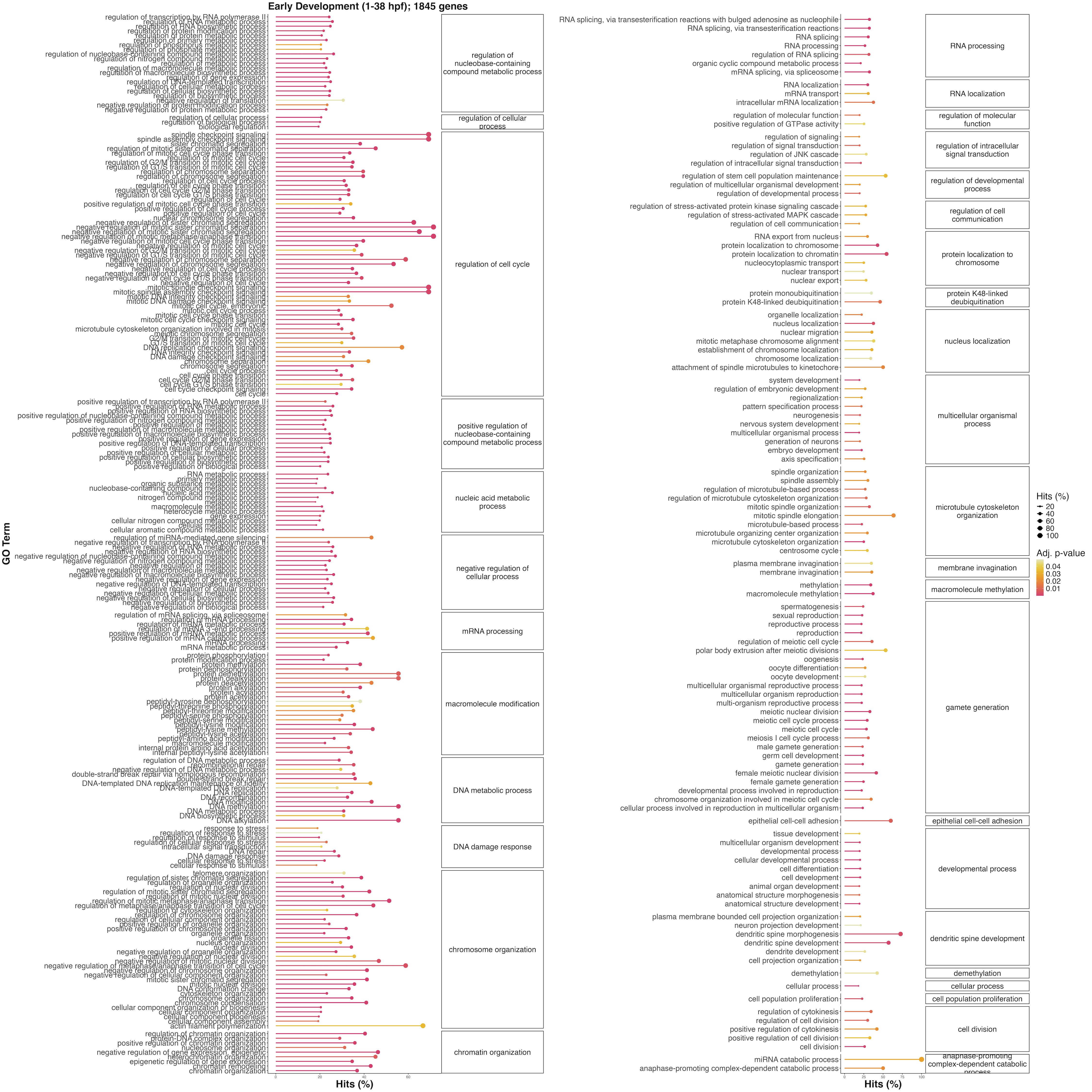
There are many terms enriched in early development. These are largely involved in cell cycle, embryonic development, cell differentiation, transcription, and related developmental terms. These likely largely represent the maternal mRNA complement provisioned to the gametes to facilitate early development.
Next plot Mid development GO terms.
go_plot_mid <- pattern_go_results %>%
  filter(pattern=="Mid")%>%
  dplyr::arrange(bh_adjust) %>%
  mutate(percHits=(numDEInCat/numInCat)*100)%>%

  ggplot(aes(x=percHits, y=term, fill=bh_adjust, colour=bh_adjust, size=percHits)) +
  facet_grid(ParentTerm ~ ., scales = "free", space='free', labeller = label_wrap_gen(width = 40, multi_line = TRUE))+
  geom_point(aes(group=term))+
  geom_segment(aes(x=0, xend=percHits, y=term, yend=term),linewidth=1) +
  scale_colour_gradientn(name = "Adj. p-value", colours = colorspace::heat_hcl(7))+
  scale_fill_gradientn(name = "Adj. p-value", colours = colorspace::heat_hcl(7))+
  scale_size(name="Hits (%)", range = c(1, 5))+
  theme_classic() +
  ylab("GO Term")+
  xlab("Hits (%)")+
  ggtitle("Mid-Development (65-163 hpf); 1696 genes")+
  theme(legend.position = "right",
        axis.text.y = element_text(size=14),
        axis.title.y = element_text(size=18, face="bold"),
        axis.title.x = element_text(size = 14, face = "bold"),
        plot.title = element_text(size = 18, face = "bold"),
        strip.text.y.right=element_text(angle=0, size=14)); go_plot_mid

ggsave(filename="Mcap2020/Figures/TagSeq/GenomeV3/DESeq/functional_enrichment/go_mid.png", go_plot_mid, width=12, height=10)
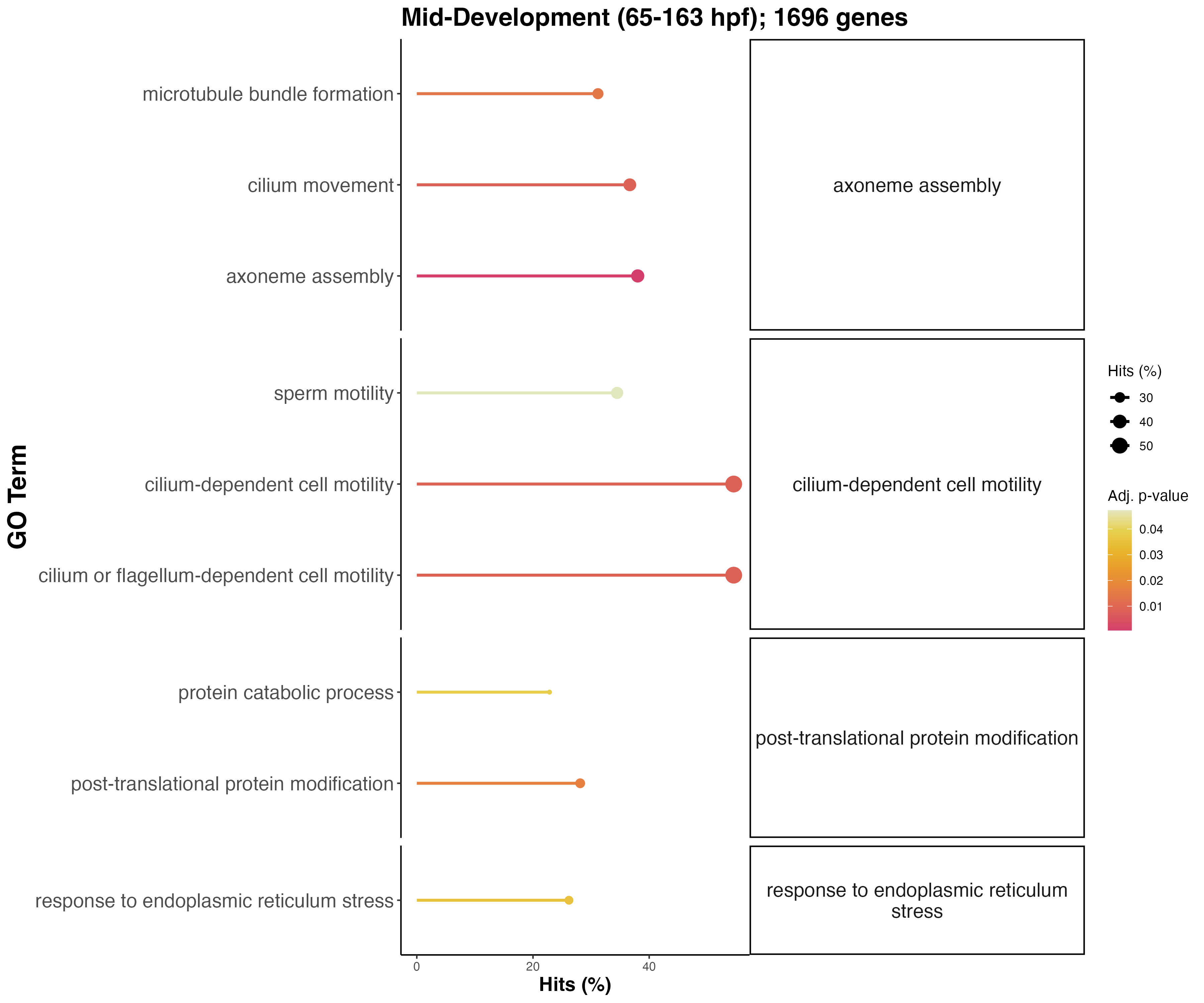
Functions in mid development are involved in motility and swimming activity, expected from swimming larvae.
Finally, plot enrichment in late development.
late_data<-pattern_go_results %>%
  filter(pattern=="Late")

# First, let's find the unique ParentTerm values
unique_late_terms <- unique(late_data$ParentTerm)

# Determine the number of unique ParentTerm values
num_unique <- length(unique_late_terms)

# Determine the midpoint for splitting into two batches
midpoint <- ceiling(num_unique / 2)
midpoint <- 7

late_data <- late_data %>%
  mutate(batch = ifelse(match(ParentTerm, unique_late_terms) <= midpoint, 1, 2))

late_data$ParentTerm <- factor(late_data$ParentTerm)
late_data$ParentTerm <- factor(late_data$ParentTerm, levels = rev(levels(late_data$ParentTerm)))

go_plot_lateA <- late_data %>%
  filter(batch=="1")%>%
  dplyr::arrange(bh_adjust) %>%
  mutate(percHits=(numDEInCat/numInCat)*100)%>%

  ggplot(aes(x=percHits, y=term, fill=bh_adjust, colour=bh_adjust, size=percHits)) +
  facet_grid(ParentTerm ~ ., scales = "free", space='free', labeller = label_wrap_gen(width = 20, multi_line = TRUE))+
  geom_point(aes(group=term))+
  geom_segment(aes(x=0, xend=percHits, y=term, yend=term),linewidth=1) +
  scale_colour_gradientn(name = "Adj. p-value", colours = colorspace::heat_hcl(7))+
  scale_fill_gradientn(name = "Adj. p-value", colours = colorspace::heat_hcl(7))+
  scale_size(name="Hits (%)", range = c(1, 5))+
  theme_classic() +
  ylab("GO Term")+
  xlab("Hits (%)")+
  ggtitle("Late Development (183-231 hpf); 2789 genes")+
  theme(legend.position = "none",
        axis.text.y = element_text(size=14),
        axis.title.y = element_text(size=18, face="bold"),
        axis.title.x = element_text(size = 14, face = "bold"),
        plot.title = element_text(size = 18, face = "bold"),
        strip.text.y.right=element_text(angle=0, size=14)); go_plot_lateA

go_plot_lateB <- late_data %>%
  filter(batch=="2")%>%
  dplyr::arrange(bh_adjust) %>%
  mutate(percHits=(numDEInCat/numInCat)*100)%>%

  ggplot(aes(x=percHits, y=term, fill=bh_adjust, colour=bh_adjust, size=percHits)) +
  facet_grid(ParentTerm ~ ., scales = "free", space='free', labeller = label_wrap_gen(width = 20, multi_line = TRUE))+
  geom_point(aes(group=term))+
  geom_segment(aes(x=0, xend=percHits, y=term, yend=term),linewidth=1) +
  scale_colour_gradientn(name = "Adj. p-value", colours = colorspace::heat_hcl(7))+
  scale_fill_gradientn(name = "Adj. p-value", colours = colorspace::heat_hcl(7))+
  scale_size(name="Hits (%)", range = c(1, 5))+
  theme_classic() +
  ylab("")+
  xlab("Hits (%)")+
  ggtitle("")+
  theme(legend.position = "right",
        axis.text.y = element_text(size=14),
        axis.title.y = element_text(size=18, face="bold"),
        axis.title.x = element_text(size = 14, face = "bold"),
        plot.title = element_text(size = 18, face = "bold"),
        strip.text.y.right=element_text(angle=0, size=14)); go_plot_lateB

go_plot_late<-plot_grid(go_plot_lateA, go_plot_lateB, ncol=2)

ggsave(filename="Mcap2020/Figures/TagSeq/GenomeV3/DESeq/functional_enrichment/go_late.png", go_plot_late, width=24, height=16)
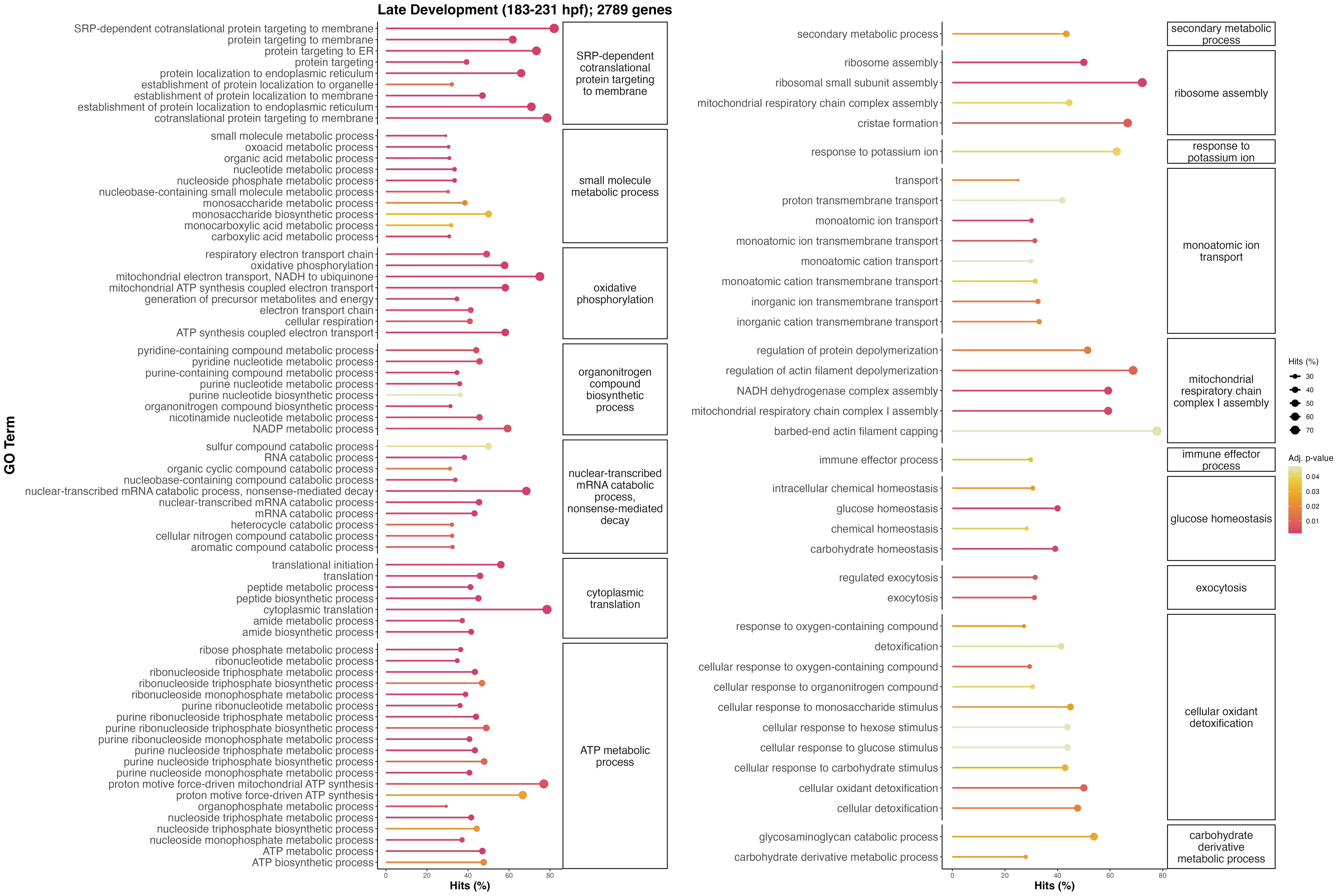
Late developmental functional enrichment results are very interesting! There is the presence of glucose homeostasis and carbohydrate metabolism, which could indicate metabolism of symbiont-derived glucose and carbohydrates fixed through photosynthesis. There is an increase in terms associated with ATP metabolism and central metabolism, indicative of increased energy metabolism and demand for energy to support settlement. We also see the presence of regulated exocytosis and response to oxygen containing compounds, which could indicate the regulation of the symbiotic relationship.
Conclusions
This analysis identified DEGs across a developmental time series in Montipora capitata. Here are my general conclusions and next steps:
- There are three large phases of molecular response across development. Early development includes embryonic development, cell growth, and transcription. Mid development (larval stages) includes genes enriched for motility and movement. Late development shows the enrichment of central metabolism, glucose response and metabolism, and symbiotic interaction functions. These general phases over development will next be informed by metabolomic responses to gain insight on shifts in specific metabolic pathways.
- There are a high number of DEGs identified, indicating strong shifts in molecular response across development to deal with drastic changes in morphology and function.
- Next, I will produce publication figures and revise the metabolomics analysis to inform these results.