


Analyzing TagSeq data with new annotation
This post details re-analyzing TagSeq data for the 2020 M. capitata developmental timeseries project to a more recent v3 genome with annotation.
Analyzing TagSeq Data with revised genome
I previously aligned sequences and generated a gene count matrix using the V1 and V2 genomes detailed in this notebook post. Results of PCA analyses are identical between verions. The previous full analysis of TagSeq data was conducted with the first version f the genome, detailed in past notebook posts.
Now, there is a more recent version of this genome published here.
This genome release includes a functional annotation (using EggNog mapper) that we can use for functional enrichment analysis. I analyzed following the steps below.
This post shows the main steps that I took. For the exact scripts used for bioinformatic analysis, view on Github here.
Bioinformatics: aligning sequences and calculating gene counts
The following are my scripts for bioinformatics steps.
Prepare GFF file
In the first round of analysis, I had a problem with alignment after the StringTie step. Many genes were returning an ID of STRG### rather than a gene name from the reference, even though the genes were aligned to the genome. In order to fix this problem, I had to change formatting in the GFF3 file. The description column (column 9) in a gff file contains information for gene or transcript names. In R, I edited the format of this file to include transcript_ID and gene_ID in this column for every gene.
The script to do this can be found on GitHub here.
1. Align sequences with HISAT2
Download sequences.
wget http://cyanophora.rutgers.edu/montipora/Montipora_capitata_HIv3.assembly.fasta.gz

wget http://cyanophora.rutgers.edu/montipora/Montipora_capitata_HIv3.genes.gff3.gz
Align using HISAT2.
#!/bin/bash
#SBATCH -t 120:00:00
#SBATCH --nodes=1 --ntasks-per-node=20
#SBATCH --export=NONE
#SBATCH --mem=200GB
#SBATCH --mail-type=BEGIN,END,FAIL #email you when job starts, stops and/or fails
#SBATCH --mail-user=ashuffmyer@uri.edu #your email to send notifications
#SBATCH --partition=putnamlab
#SBATCH --error="alignV3_error" #if your job fails, the error report will be put in this file
#SBATCH --output="alignV3_output" #once your job is completed, any final job report comments will be put in this file
#SBATCH -D /data/putnamlab/ashuffmyer/mcap-2020-tagseq/sequences

# load modules needed
module load HISAT2/2.2.1-foss-2019b
module load SAMtools/1.9-foss-2018b

#unzip reference genome
#gunzip Montipora_capitata_HIv3.assembly.fasta.gz

# index the reference genome for Montipora capitata output index to working directory
hisat2-build -f /data/putnamlab/ashuffmyer/mcap-2020-tagseq/sequences/Montipora_capitata_HIv3.assembly.fasta ./Mcapitata_ref_v3 # called the reference genome (scaffolds)
echo "Referece genome indexed. Starting alingment" $(date)

# This script exports alignments as bam files
# sorts the bam file because Stringtie takes a sorted file for input (--dta)
# removes the sam file because it is no longer needed
array=($(ls clean*)) # call the clean sequences - make an array to align
for i in ${array[@]}; do
        sample_name=`echo $i| awk -F [.] '{print $2}'`
	hisat2 -p 8 --dta -x Mcapitata_ref_v3 -U ${i} -S ${sample_name}.sam
        samtools sort -@ 8 -o ${sample_name}.bam ${sample_name}.sam
    		echo "${i} bam-ified!"
        rm ${sample_name}.sam
done
This generates a .bam file for each sequence file.
2. Assemble with StringTie2
Sequence .bam files were then assembled with StringTie2.
#!/bin/bash
#SBATCH -t 120:00:00
#SBATCH --nodes=1 --ntasks-per-node=20
#SBATCH --export=NONE
#SBATCH --mem=200GB
#SBATCH --mail-type=BEGIN,END,FAIL #email you when job starts, stops and/or fails
#SBATCH --mail-user=ashuffmyer@uri.edu #your email to send notifications
#SBATCH --account=putnamlab
#SBATCH --error="stringtieV3_error" #if your job fails, the error report will be put in this file
#SBATCH --output="stringtieV3_output" #once your job is completed, any final job report comments will be put in this file
#SBATCH -D /data/putnamlab/ashuffmyer/mcap-2020-tagseq/sequences

#load packages
module load StringTie/2.1.4-GCC-9.3.0

#Transcript assembly: StringTie

array=($(ls *.bam)) #Make an array of sequences to assemble

for i in ${array[@]}; do #Running with the -e option to compare output to exclude novel genes. Also output a file with the gene abundances
        sample_name=`echo $i| awk -F [_] '{print $1"_"$2"_"$3}'`
	stringtie -p 8 -e -B -G Montipora_capitata_HIv3.genes.gff3 -A ${sample_name}.gene_abund.tab -o ${sample_name}.gtf ${i}
        echo "StringTie assembly for seq file ${i}" $(date)
done
echo "StringTie assembly COMPLETE, starting assembly analysis" $(date)
3. Generate gene count matrix with Prep DE
Use Prep DE to generate a matrix of gene counts.
#!/bin/bash
#SBATCH -t 120:00:00
#SBATCH --nodes=1 --ntasks-per-node=20
#SBATCH --export=NONE
#SBATCH --mem=200GB
#SBATCH --mail-type=BEGIN,END,FAIL #email you when job starts, stops and/or fails
#SBATCH --mail-user=ashuffmyer@uri.edu #your email to send notifications
#SBATCH --account=putnamlab
#SBATCH --error="stringtieV3_error" #if your job fails, the error report will be put in this file
#SBATCH --output="stringtieV3_output" #once your job is completed, any final job report comments will be put in this file
#SBATCH -D /data/putnamlab/ashuffmyer/mcap-2020-tagseq/sequences

#load packages
module load Python/2.7.15-foss-2018b #Python
module load StringTie/2.1.4-GCC-9.3.0

#Transcript assembly: StringTie
module load GffCompare/0.12.1-GCCcore-8.3.0

#Transcript assembly QC: GFFCompare

#make gtf_list.txt file
ls AH*.gtf > gtf_list.txt

stringtie --merge -p 8 -G Montipora_capitata_HIv3.genes.gff3 -o Mcapitata_merged.gtf gtf_list.txt #Merge GTFs to form $
echo "Stringtie merge complete" $(date)

gffcompare -r Montipora_capitata_HIv3.genes.gff3 -G -o merged Mcapitata_merged.gtf #Compute the accuracy and pre$
echo "GFFcompare complete, Starting gene count matrix assembly..." $(date)

#make gtf list text file
for filename in AH*.gtf; do echo $filename $PWD/$filename; done > listGTF.txt

python ../scripts/prepDE.py -g Mcapitata_gene_count_matrix_V3.csv -i listGTF.txt #Compile the gene count matrix
echo "Gene count matrix compiled." $(date)
Rename and move gene count matrix off of server
scp ashuffmyer@ssh3.hac.uri.edu:/data/putnamlab/ashuffmyer/mcap-2020-tagseq/Mcapitata_gene_count_matrix_V3.csv ~/MyProjects/EarlyLifeHistory_Energetics/Mcap2020/Output/TagSeq
We will then use the file Mcapitata_gene_count_matrix_V3.csv for analysis of gene expression.
Alignment rates of our sequences were approx. 70%, similar to previous genome versions.
Conduct WGCNA analysis
Once I obtained a revised gene count matrix using the new genome, I re-ran the WGCNA analysis to determine which genes are associated with lifestage time points. In this post, I will detail the main steps used and if the analysis deviated from previous analysis.
Scripts for this analysis are on GitHub here.
1. Filtering and preparing data
First, we load the gene count matrix and remove genes that were not expressed in any of our samples. The new M. capitata genome had 54,384 genes. After removing genes that were not expressed, we were left with 34,223 genes in our dataset. It is expected that we will not capture the every possible gene in our dataset due to the specific environmental conditions and lifestages of our samples (e.g., we likely will not see genes related to gametogenesis to calcification that we would see in adult tissues).
Next, we filtered genes using the pOverA function in the genefilter package: filterfun(pOverA(0.07,10)).
In this analysis, we used a pOverA of (0.07,10). This specifies the minimum count for a proportion of samples for each gene for that gene to be retained in analysis. Here, we are using a pOverA of 0.07. This is because we have 38 samples with a minimum of n=3 samples per lifestage. Therefore, we will accept genes that are present in 3/38 = 0.07 of the samples because we are testing for different expression by life stage. We are further setting the minimum count of genes to 10, such that 7% of the samples must have a gene count of >10 in order for the gene to remain in the data set.
After filtering we have 11,475 genes in our dataset.
2. Construct DESeq2 object
I used the following code to construct a DESeq2 dataset:
gdds <- DESeqDataSetFromMatrix(countData = gcount_filt,
                              colData = metadata_ordered,
                              design = ~lifestage)
Where gcount_filt is our filtered gene count matrix and metadata_ordered is a dataframe of metadata ordered in the same order as samples listed in the count matrix. We are testing the design by lifestage grouping. I then applied a variance stabilizing transformation (VST) to the gene counts DESeq2 object.
gvst <- vst(gdds, blind=FALSE)
3. View multivariate gene expression and run PERMANOVA
Next, I vizualized gene expression patterns across lifestages with a PERMANOVA. I used the vegan package to scale and center our VST-transformed matrix and test using a PERMANOVA.
scaled_test <-prcomp(test[c(1:11475)], scale=TRUE, center=TRUE)
fviz_eig(scaled_test)

# scale data
vegan <- scale(test[c(1:11475)])

# PerMANOVA
permanova<-adonis2(vegan ~ Lifestage, data = test, method='eu')
permanova
The results of the PERMANOVA show significant separation in gene expression between lifestages.
Permutation test for adonis under reduced model
Terms added sequentially (first to last)
Permutation: free
Number of permutations: 999

adonis2(formula = vegan ~ Lifestage, data = test, method = "eu")
          Df SumOfSqs      R2      F Pr(>F)
Lifestage  9   318674 0.75057 9.3618  0.001 ***
Residual  28   105901 0.24943
Total     37   424575 1.00000
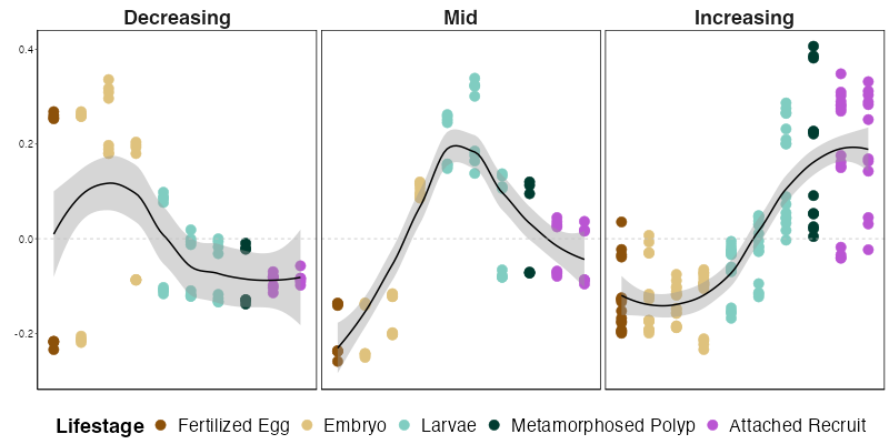
Visually, a PCA of this data looks like this:
There is clear separation in early development(brown=eggs, yellow=embryos), mid development (cyan=larvae), and late development (green=metamorphosed polyps, pink=attached recruits).
Now we can look into which genes are correlated with life stages with a WGCNA analysis.
4. Conduct WGCNA
I conducted a WGCNA analysis using the Dynamic Tree Cut approach using step-by-step network construction and module detection. Analysis based on resources from the Horvath Lab and Erin Chille’s scripts.
I first examine and select a soft thresholding power using a scale-free topology fit index of R^2=0.90. The lowest recommended is 0.8 (Langfelder and Horvath). We used 0.9 to maximize the model fit. In this analysis, the soft thresholding power was 5, the same as in previous analysis.
I then used a signed network to calculate a topological overlap matrix and dissimiliarity.
adjacency=adjacency(datExpr, power=softPower,type="signed")
TOM= TOMsimilarity(adjacency,TOMType = "signed")
dissTOM= 1-TOM
I then identified modules using dynamicTreeCut dynamic module detection. More information on this method can be found here.
minModuleSize = 30
dynamicMods = cutreeDynamic(dendro = geneTree, distM = dissTOM,
deepSplit = TRUE, pamRespectsDendro = FALSE,
minClusterSize = minModuleSize)
Minimum module size is set to 30 in this analysis.
12 modules were identified, with the lower module numbers as bigger modules and higher numbers are modules with less genes.
dynamicMods
   1    2    3    4    5    6    7    8    9   10   11   12
3536 3073 2352  737  622  603  299   56   54   52   52   39
Module eigengenes (essentially expression levels of each module) are calculated and modules are then clustered. The purpose of clustering is to identify modules with similar expression patterns that can be merged.
MEList = moduleEigengenes(datExpr, colors = dynamicColors, softPower = 5)
MEs = MEList$eigengenes
MEDiss = 1-cor(MEs)
METree = flashClust(as.dist(MEDiss), method = "average")
Modules were merged if they were >85% similar.
MEDissThres= 0.15
merge= mergeCloseModules(datExpr, dynamicColors, cutHeight= MEDissThres, verbose =3)
We had 12 modules before merging and this was reduced to 9 after merging.
mergedColors
   1    2    3    5    6    7    8    9   12
3536 3073 3089  674  603  299  108   54   39
I then related these modules to lifestage by assigning either a 1 if module was associated with a lifestage or 0 if it was not. The “trait” in this analysis is considered the ontogenetic order of lifestages. This treats lifestage as a binary variable so that we can calculate correlation to lifestage.
metadata_ordered$num <- c("1")
allTraits <- as.data.frame(pivot_wider(metadata_ordered, names_from = lifestage, values_from = num, id_cols = sample_id))
allTraits[is.na(allTraits)] <- c("0")
rownames(allTraits) <- allTraits$sample_id
datTraits <- allTraits[,c(-1)]
datTraits

moduleTraitCor = cor(MEs, datTraits, use = "p");
moduleTraitPvalue = corPvalueStudent(moduleTraitCor, nSamples);
Colors=sub("ME","", names(MEs))

moduleGeneCor=cor(MEs,datExpr)
moduleGenePvalue = corPvalueStudent(moduleGeneCor, nSamples)
Using these values of association to lifestage, we can now get to the fun part! We can view a heatmap generated with the complexHeatmap package to view associations of modules with lifestage.
This shows that there are 3 general groupings of modules - those associated with early development (eggs, embryos), mid development (larvae, late embryos), and late development (late larvae, polyps, recruits).
In this figure, the red squares are positively associated with lifestage and blue are negatively associated. Bold indicates statistical significance indicated by p-values.
5. View module eigengene over development
I also visualized the expression of each module over development to view patterns.

There are clear expression patterns over development that vary by module. Some are higher in early, mid, or late development.
Conduct functional enrichment analysis in GOseq
The generated list of genes and association with modules and lifestages is then used for functional enrichment. This version of the genome includes a Gene Ontology (GO) functional annotation and a KEGG annotation. These files are avaiable for download here.
I performed functional enrichment in the goseq package.
1. Calculate gene lengths
GOSeq requires information about the gene length to calculate bias. I calculated gene lengths from the gff3 file.
#import file
gff <- import("Mcap2020/Data/TagSeq/Montipora_capitata_HIv3.genes.gff3")
transcripts <- subset(gff, type == "transcript") #keep only transcripts
transcripts_gr <- makeGRangesFromDataFrame(transcripts, keep.extra.columns=TRUE) #extract length information
transcript_lengths <- width(transcripts_gr) #isolate length of each gene
seqnames<-transcripts_gr$ID #extract list of gene id
lengths<-cbind(seqnames, transcript_lengths)
lengths<-as.data.frame(lengths) #convert to data frame
2. Run GOSeq by module
I ran functional enrichment analysis first at the level of each module.
This analysis was run in a loop specified below for each module. This script reads in vectors of all possible genes, a vector of the genes in the respective module, a vector of gene lengths for GOSeq anaysis, and a list of the GO terms associated with each gene read in from the functional annotation file (EggNog_results). In this script, the GO terms are formatted to have one GO term per row. In some cases, there are dozens of GO terms per gene.
GOSeq was run in a loop for each module:
module_vector<-c(levels(geneInfo$Module))

for (module in module_vector) {

    ### Generate vector with names of all genes
    ALL.vector <- c(geneInfo$gene_id)

    ### Generate length vector for all genes
    LENGTH.vector <- as.integer(geneInfo$Length)

    ### Generate vector with names in just the module we are analyzing
    ID.vector <- geneInfo%>%
      filter(Module==module)%>%
      #get_rows(.data[[module]]))%>%
      pull(gene_id)

    ##Get a list of GO Terms for each module
    GO.terms <- geneInfo%>%
      filter(Module==module)%>%
      #filter(get_rows(.data[[module]]))%>%
      dplyr::select(gene_id, Annotation.GO.ID)

    ##Format to have one goterm per row with gene ID repeated
    split <- strsplit(as.character(GO.terms$Annotation.GO.ID), ";")
    split2 <- data.frame(v1 = rep.int(GO.terms$gene, sapply(split, length)), v2 = unlist(split))
    colnames(split2) <- c("gene", "Annotation.GO.ID")
    GO.terms<-split2

    ##Construct list of genes with 1 for genes in module and 0 for genes not in the module
    gene.vector=as.integer(ALL.vector %in% ID.vector)
    names(gene.vector)<-ALL.vector#set names

    #weight gene vector by bias for length of gene
    pwf<-nullp(gene.vector, ID.vector, bias.data=LENGTH.vector)

    #run goseq using Wallenius method for all categories of GO terms
    GO.wall<-goseq(pwf, ID.vector, gene2cat=GO.terms, test.cats=c("GO:BP", "GO:MF", "GO:CC"), method="Wallenius", use_genes_without_cat=TRUE)

    GO <- GO.wall[order(GO.wall$over_represented_pvalue),]
    colnames(GO)[1] <- "GOterm"

    #adjust p-values
    GO$bh_adjust <-  p.adjust(GO$over_represented_pvalue, method="BH") #add adjusted p-values

    #Filtering for p < 0.0001
    GO <- GO %>%
        dplyr::filter(bh_adjust<0.001) %>%
        dplyr::arrange(., ontology, bh_adjust)

    #Write file of results
    write_csv(GO, file = paste0("Mcap2020/Output/TagSeq/GenomeV3/GOSeq/goseq_module", module, ".csv"))

}
In this analysis, I conducted functional enrichment for BP, MF, and CC ontologies.
When I first ran this analysis, I found that there were thousands of GO terms enriched in the larger gene modules. This was far too many to visualize or analyze further, so I increased the adjusted p-value cut off to <0.001. I tried several iterations of these thresholds and found that a majority of the GO terms were highly highly significant below the 0.001 p-value threshold. We can therefore proceed with these enriched terms that are highly significantly enriched.
I then ran a loop to generate a plot for each ontology level for each module.
In this next part of the analysis, I followed several steps to again reduce the number of GO terms that we are visualizing (there were SO many prior to these additional steps):
- Reduce p-value cut off to <0.001 (above)
- Use the
rrvgopackage to remove highly redundant GO terms (using a C. elegans database and threshold of 0.7 for medium sensitivity) - Only include GO term categories with at least 10 genes included
- Finally, filter Parent Terms by keywords that we are interested in for this paper
The script was as follows:
module_vector<-c(levels(geneInfo$Module))
ontologies<-c("BP", "MF")

#add vector for terms of interest to reduce number of GO terms
keywords<-c("metabolism", "carbon", "carbohydrate", "lipid", "fatty", "apoptosis", "death", "symbiosis", "regulation of cell communication", "trans membrane transport", "transmembrane", "glucose", "organic substance transport", "response to stress", "antioxidant")

for (module in module_vector) {

  for (category in ontologies) {

    #Read relevant file of results from goseq analysis
    go_results<-read_csv(file = paste0("Mcap2020/Output/TagSeq/GenomeV3/GOSeq/goseq_module", module, ".csv"))

    go_results<-go_results%>%
      filter(ontology==category)%>%
      filter(bh_adjust != "NA") %>%
      filter(numInCat>10)%>%
      arrange(., bh_adjust)

      #Reduce/collapse GO term set with the rrvgo package
      simMatrix <- calculateSimMatrix(go_results$GOterm,
                                orgdb="org.Ce.eg.db", #c. elegans database
                                ont=category,
                                method="Rel")
    #calculate similarity
    scores <- setNames(-log(go_results$bh_adjust), go_results$GOterm)
    reducedTerms <- reduceSimMatrix(simMatrix,
                                scores,
                                threshold=0.7,
                                orgdb="org.Ce.eg.db")

    #keep only the goterms from the reduced list
    go_results<-go_results%>%
      filter(GOterm %in% reducedTerms$go)

    #add in parent terms to list of go terms
    go_results$ParentTerm<-reducedTerms$parentTerm[match(go_results$GOterm, reducedTerms$go)]

    go_results<-go_results%>%
      filter(grepl(paste(keywords, collapse="|"), ParentTerm))

    #plot significantly enriched GO terms by Slim Category faceted by slim term
  GO.plot <-  ggplot(go_results, aes(x = ontology, y = term)) +
    geom_point(aes(size=bh_adjust)) +
    scale_size(name="Over rep. p-value", trans="reverse")+
    facet_grid(ParentTerm ~ ., scales = "free_y", labeller = label_wrap_gen(width = 5, multi_line = TRUE))+
    theme_bw() + theme(panel.border = element_blank(), panel.grid.major = element_blank(),
    panel.grid.minor = element_blank(), axis.line = element_line(colour = "black"),
    strip.text.y = element_text(angle=0, size = 10),
    strip.text.x = element_text(size = 20),
    axis.text = element_text(size = 8),
    axis.title.x = element_blank(),
    axis.title.y = element_blank())

ggsave(filename=paste0("Mcap2020/Figures/TagSeq/GenomeV3/GOSeq/GOenrich_Module", module, "_", category, ".png"), plot=GO.plot, dpi=300, width=8, height=49, units="in")

  }
}
This generates plots of GO terms with numbers of GO terms that are reasonable to work with. We can further explore other key words and thresholds to investigate other aspects of this dataset. Here, I am most interested in carbohydrate and lipid metabolism, transport and communication.
An example of plots looks like this:
Below we will approach this analysis to make plots that are visually helpful and reduce the data further.
3. Run GOSeq by ontogenetic pattern
To view patterns across ontogeny, I grouped modules into ontogenetic patterns. We saw in the WGCNA heatmap that there are groups of modules associated with early, mid, or late development.
I used the eigengene plot above to determine which modules fall into each pattern.
Increase over development = 12, 3, 5, 9
Decrease over development = 1, 8
Peak in mid-development = 2, 6
Module 7 only peaks in one stage so we won’t include it here in the patterns.
When summarized, the expression of modules in these patterns looks like this. We can see that expression generally follows these three distinct patterns. There are some modules in early development that are high in some embryonic stages, but low in others, generating a few points that are low in early development in that pattern. I will be looking into this in more detail to see if we need to split up this pattern even more.
I then took the same approach to run a loop to conduct GOSeq for each of these patterns, rather than at the module level.
increase<-c("12", "3", "5", "9")
decrease<-c("1", "8")
mid<-c("2", "6")

geneInfo<-geneInfo%>%
  mutate(Pattern=if_else(Module %in% increase, "Increasing", "NA"))%>%
  mutate(Pattern=if_else(Module %in% decrease, "Decreasing", Pattern))%>%
  mutate(Pattern=if_else(Module %in% mid, "Mid", Pattern))

pattern_vector<-c("Increasing", "Decreasing", "Mid")

for (pattern in pattern_vector) {

    ### Generate vector with names of all genes
    ALL.vector <- c(geneInfo$gene_id)

    ### Generate length vector for all genes
    LENGTH.vector <- as.integer(geneInfo$Length)

    ### Generate vector with names in just the module we are analyzing
    ID.vector <- geneInfo%>%
      filter(Pattern==pattern)%>%
      #get_rows(.data[[module]]))%>%
      pull(gene_id)

    ##Get a list of GO Terms for each module
    GO.terms <- geneInfo%>%
      filter(Pattern==pattern)%>%
      #filter(get_rows(.data[[module]]))%>%
      dplyr::select(gene_id, Annotation.GO.ID)

    ##Format to have one goterm per row with gene ID repeated
    split <- strsplit(as.character(GO.terms$Annotation.GO.ID), ";")
    split2 <- data.frame(v1 = rep.int(GO.terms$gene, sapply(split, length)), v2 = unlist(split))
    colnames(split2) <- c("gene", "Annotation.GO.ID")
    GO.terms<-split2

    ##Construct list of genes with 1 for genes in module and 0 for genes not in the module
    gene.vector=as.integer(ALL.vector %in% ID.vector)
    names(gene.vector)<-ALL.vector#set names

    #weight gene vector by bias for length of gene
    pwf<-nullp(gene.vector, ID.vector, bias.data=LENGTH.vector)

    #run goseq using Wallenius method for all categories of GO terms
    GO.wall<-goseq(pwf, ID.vector, gene2cat=GO.terms, test.cats=c("GO:BP", "GO:MF", "GO:CC"), method="Wallenius", use_genes_without_cat=TRUE)

    GO <- GO.wall[order(GO.wall$over_represented_pvalue),]
    colnames(GO)[1] <- "GOterm"

    #adjust p-values
    GO$bh_adjust <-  p.adjust(GO$over_represented_pvalue, method="BH") #add adjusted p-values

    #Filtering for p < 0.01
    GO <- GO %>%
        dplyr::filter(bh_adjust<0.0001) %>%
        dplyr::arrange(., ontology, bh_adjust)

    #Write file of results
    write_csv(GO, file = paste0("Mcap2020/Output/TagSeq/GenomeV3/GOSeq/goseq_pattern_", pattern, ".csv"))

}
The cutoffs and thresholds are the same as for our module analysis above.
I then plotted the results for each pattern using the same rrvgo approach.
For this analysis, I am visualizing only the BP (biological process) ontology.
First, I plotted functional enrichment terms related to Carbohdyrate Metabolism:
#bring in dataframes and bind them together
file1<-read_csv("Mcap2020/Output/TagSeq/GenomeV3/GOSeq/goseq_pattern_Increasing.csv")%>%mutate(pattern="Increasing")
file2<-read_csv("Mcap2020/Output/TagSeq/GenomeV3/GOSeq/goseq_pattern_Decreasing.csv")%>%mutate(pattern="Decreasing")
file3<-read_csv("Mcap2020/Output/TagSeq/GenomeV3/GOSeq/goseq_pattern_Mid.csv")%>%mutate(pattern="Mid")
patterns_df<-rbind(file1, file2, file3)

patterns_df$pattern<-factor(patterns_df$pattern, levels=c("Decreasing", "Mid", "Increasing"))

category<-c("BP")

#add vector for terms of interest to reduce number of GO terms
carbs<-c("carbohydrate")

    #Read relevant file of results from goseq analysis
    go_results<-patterns_df

    go_results<-go_results%>%
      filter(ontology==category)%>%
      filter(bh_adjust != "NA") %>%
      filter(numInCat>10)%>%
      arrange(., bh_adjust)

    #Reduce/collapse GO term set with the rrvgo package
      simMatrix <- calculateSimMatrix(go_results$GOterm,
                                orgdb="org.Ce.eg.db", #c. elegans database
                                ont=category,
                                method="Rel")
    #claculate similarity
    scores <- setNames(-log(go_results$bh_adjust), go_results$GOterm)
    reducedTerms <- reduceSimMatrix(simMatrix,
                                scores,
                                threshold=0.7,
                                orgdb="org.Ce.eg.db")

    #keep only the goterms from the reduced list
    go_results<-go_results%>%
      filter(GOterm %in% reducedTerms$go)

    #add in parent terms to list of go terms
    go_results$ParentTerm<-reducedTerms$parentTerm[match(go_results$GOterm, reducedTerms$go)]

    go_results<-go_results%>%
      filter(grepl(paste(carbs, collapse="|"), ParentTerm))

    #plot significantly enriched GO terms by Slim Category faceted by slim term
  GO.plot.carb <-  ggplot(go_results, aes(x = pattern, y = term)) +
    geom_point(aes(size=bh_adjust, colour=pattern)) +
    scale_size(name="Over rep. p-value", trans="reverse", range=c(3,6))+
    facet_grid(ParentTerm ~ ., scales = "free", space='free', labeller = label_wrap_gen(width = 6, multi_line = TRUE))+
    scale_colour_manual(values=c("lightgray", "darkgray", "black"), guide=FALSE)+
    xlab("Ontogenetic Pattern")+
    ggtitle("Carbohydrate Metabolism")+
    theme_bw() +
    theme(panel.border = element_blank(),
          panel.grid.major = element_blank(),
          panel.grid.minor = element_blank(), axis.line = element_line(colour = "black"),
          strip.background =element_rect(fill="white"),
          strip.text.y = element_text(angle=0, size = 18, face="bold"),
          strip.text.x = element_text(size = 16),
          axis.text.x = element_text(size = 20, angle=45, hjust=1),
          axis.text.y = element_text(size = 16),
          axis.title.x = element_text(size = 22, face="bold"),
          legend.text=element_text(size=16),
          title=element_text(size=22, face="bold"),
          plot.title = element_text(hjust = 0.1),
          axis.title.y = element_blank())

ggsave(filename=paste0("Mcap2020/Figures/TagSeq/GenomeV3/GOSeq/GOenrich_AllPatterns_Carbohdyrate.png"), plot=GO.plot.carb, dpi=300, width=13, height=18, units="in")
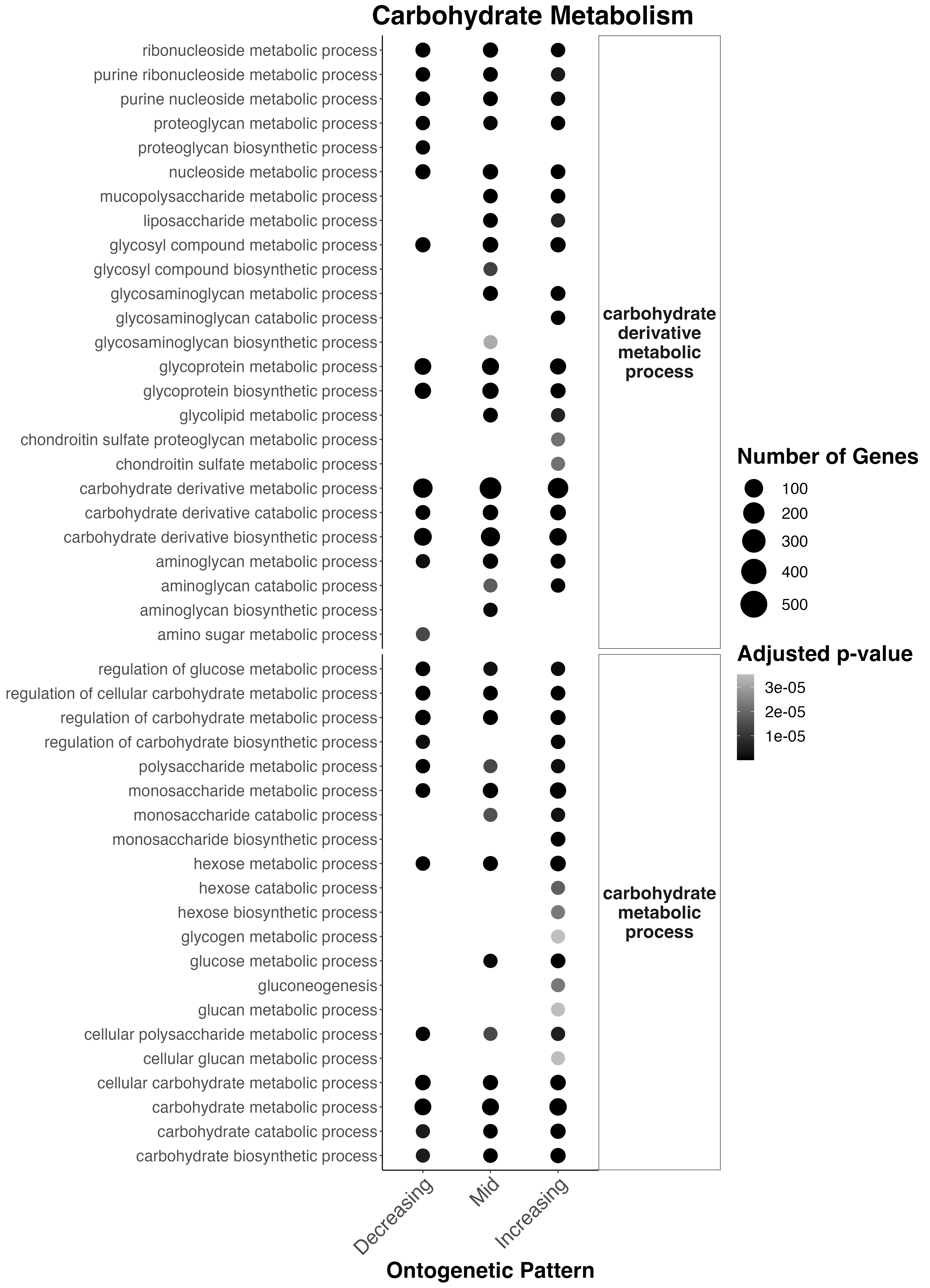
Interesting results
- Carbohydrate derivative metabolism occurs across development. Interestingly amino sugar metabolism only occurs early in development.
- Several other carb. derivative metabolic processes start in mid and late development including liposaccharide metabolism, glycosyl compound metabolic processes, glycolipid metabolism, condroitin sulfate metabolism, and aminoglycan metabolism.
- Carbohydrate metabolism regulation occurs throughout development with monosaccharide metabolism present throughout. Interestingly, hexose metabolism (glucose, fructose, etc) is only found late in development.
- Glucose metabolism occurs in mid to late development.
- Gluconeogenesis occurs in late development.
This aligns with out metabolomic data suggesting a transition and increase towards higher metabolism of carbohdyrates (which may be coming from symbionts) later in development.
I used the same code/approach to view functional enrichment of lipid metabolism and communication/transport.
I used the following key words for these categories.
lipids<-c("lipid", "fatty")
symbiosis<-c("regulation of cell communication", "transmembrane transport", "transmembrane", "organic substance transport", "antioxidant", "oxygen")
Lipid metabolism across these ontogenetic patterns looks like this:
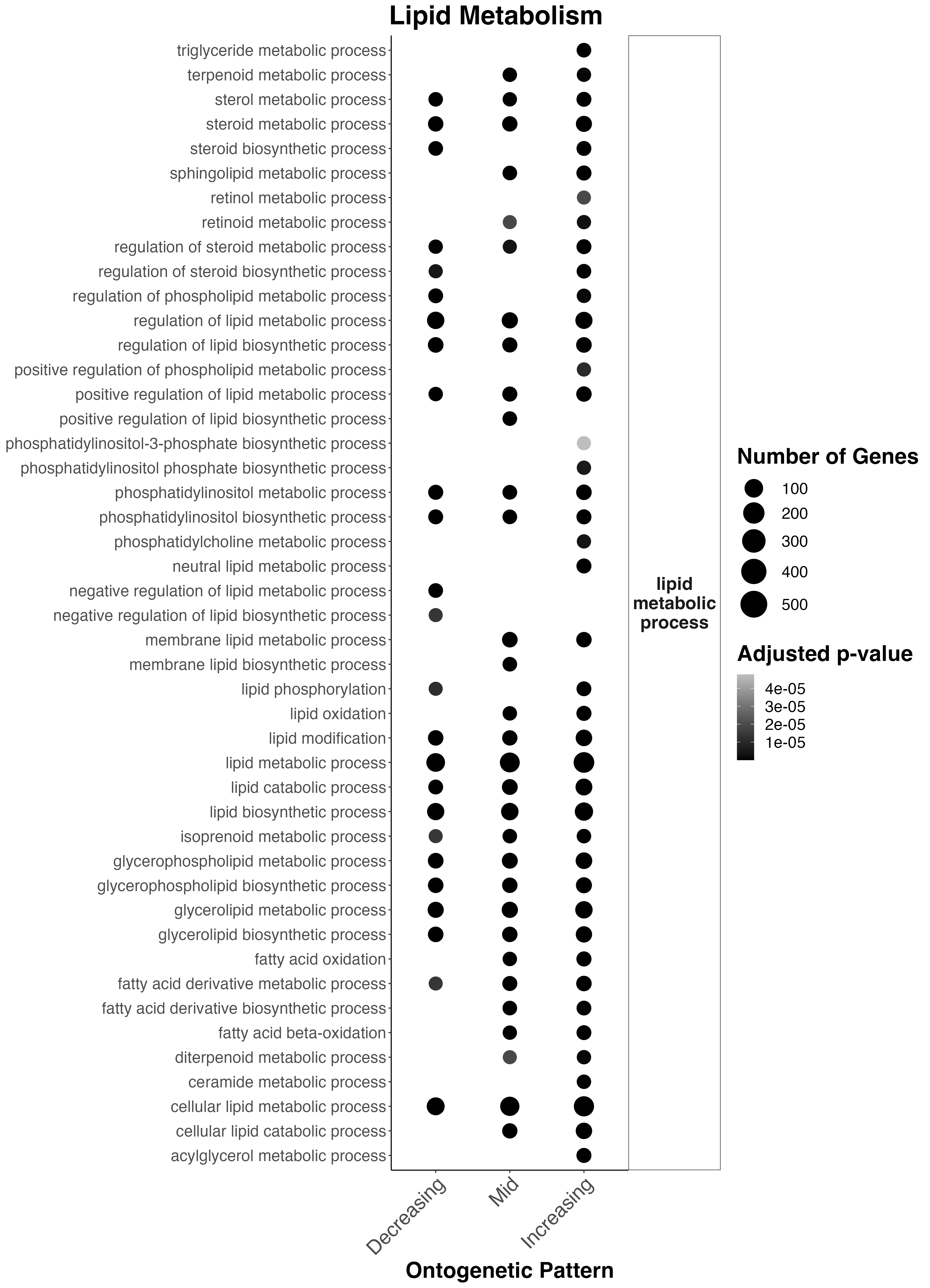
Interesting results
- Sterol metabolism, regulation of lipid metabolism, phosphatidylinositol metabolism, lipid metabolism, glycerophospholipid metabolism, and cellular lipid metabolism occur throughout development.
- There is an increase in lipid metabolism in mid and late development in sphingolipid metabolism, retinoid metabolism, positive regulation of lipid biosynthesis, membrane lipid metabolism, lipid oxidation, fatty acid oxidation, and fatty acid metabolism.
- In late development, there is an increase in triglyceride metabolism, positive regulation of phospholipid metabolism, neutral lipid metabolism, and acylglyercol metabolism.
This suggests that there is increased metabolism of potential symbiont-derived fatty acids occurs in mid-late development and there are shifts in the allocation/metabolism of energy reserves along develoment.
Finally, communication/transport terms look like this:
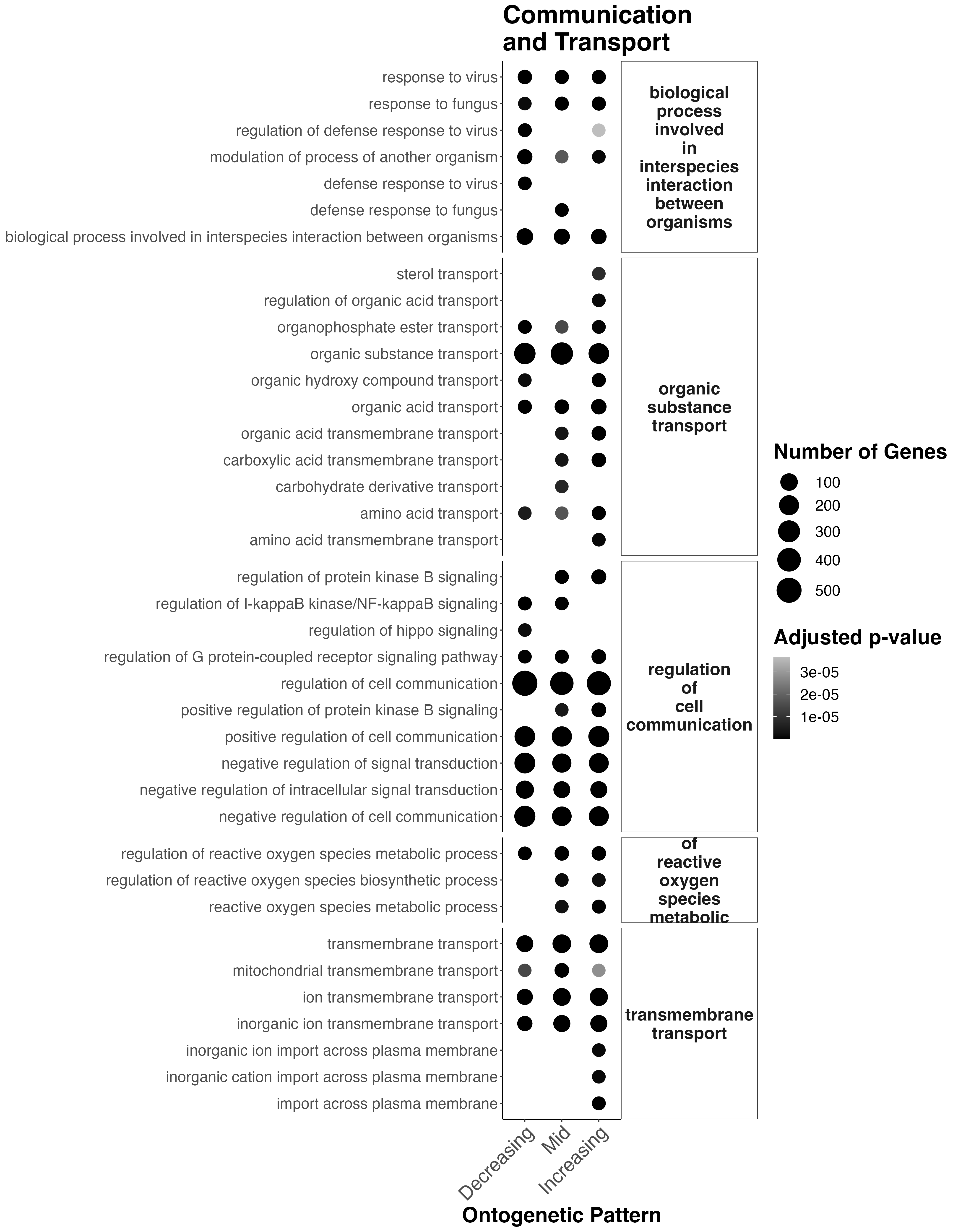
Interesting results
- Throughout development, there is transport and cell communication pathways active.
- In mid development, there starts to be an increase in organic acid and carboxylic acid transmembrane transport and carbohydrate derivative transmembrane transport.
- There are shifts in development in protein kinase B signaling pathways which is involved with cell cycle progression and proliferation, cell survival, protein synthesis, and cell growth (higher in mid-late development). This could relate to symbiont population growth.
- In mid-late development there is increased reactive oxygen species metabolism, which could be due to increased symbiont populations.
- In late development there is increased import across plasma membranes.
This suggests that the coral is responding/changing communication and transport pathways across development which may relate to shifts in symbiont metabolism/translocation/population growth.
5. Next steps
I am next going to revise methods and results of our manuscript to reflect this revised analysis and dig into the details of the functional enrichment results.