This post details recent updates to the Montipora capitata developmental time series 16S analysis.

See these notebook posts for the mothur bioinformatic pipeline that we used and initial analyses in R.

Overview

The dataset we are analyzing was collected across early life stages of M. capitata in Hawaii in 2020 including egg, embryo, larval, metamorphosed polyp, and attached recruit stages. See my notebook page for more information on the project.

Following bioinformatics steps above in the mothur pipeline, we lost several samples due to low sequence counts during subsampling. For this analysis, we are working with the following lifestages:

• Embryos (38 hpf)
• Embryos (65 hpf)
• Larvae (93 hpf)
• Larvae (163 hpf)
• Larvae (231 hpf)
• Metamorphosed Polyps (231 hpf)
• Attached Recruits (183 hpf)
• Attached Recruits (231 hpf)

In this analysis, my goals were to vizualize:

1. Alpha diversity (diversity metrics)
2. Beta diversity (NMDS)
3. Relative abundance of microbial taxa

Working scripts for this analysis can be found on GitHub here.

1. Alpha diversity

Data for this project were analyzed using the phyloseq package in R (v1.42.0). I first visualized alpha diveristy calculated using the Shannon and Inverse Simpson indices.

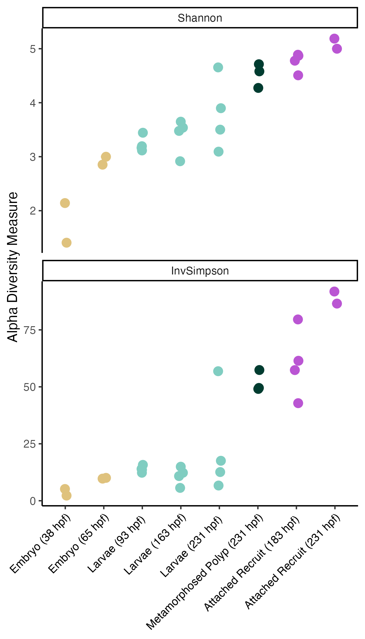
These data indicate that alpha diversity increases with development and is highest in the attached recruit stages.

An ANOVA analysis shows significant variation in alpha diversity by lifestage.

summary(aov(InvSimpson~lifestage, data=alpha_rare))

            Df Sum Sq Mean Sq F value  Pr(>F)    
lifestage    7  16906  2415.1   17.46 1.3e-06 ***
Residuals   17   2351   138.3  

summary(aov(Shannon~lifestage, data=alpha_rare))

            Df Sum Sq Mean Sq F value   Pr(>F)    
lifestage    7 20.247  2.8925   22.31 2.16e-07 ***
Residuals   17  2.204  0.1296   

Next, I plotted beta diversity using a non-metric multidimensional scaling analysis (NMDS).

2. Beta diversity/NMDS

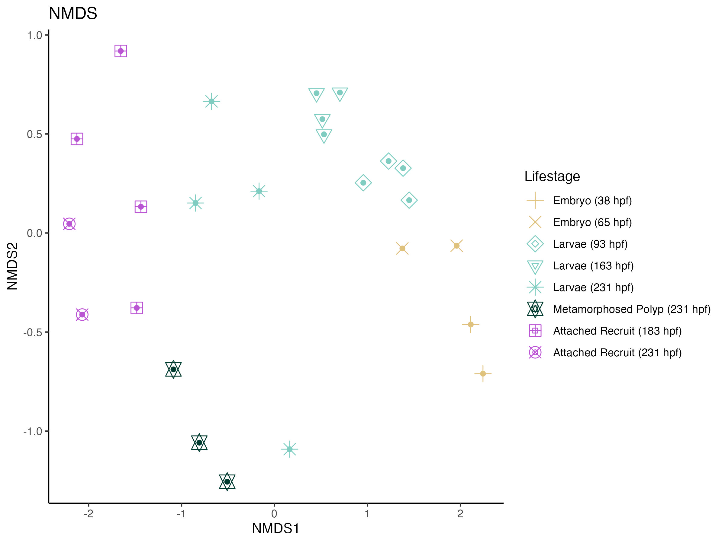
I used an NMDS to visualize beta diversity across lifestages.

Square root transformation
Wisconsin double standardization
Run 0 stress 0.09573264 
Run 1 stress 0.1160347 
Run 2 stress 0.1140127 
Run 3 stress 0.1136736 
Run 4 stress 0.09436607 
... New best solution
... Procrustes: rmse 0.01242604  max resid 0.04919756 
Run 5 stress 0.09436607 
... New best solution
... Procrustes: rmse 2.287365e-05  max resid 9.523698e-05 
... Similar to previous best
Run 6 stress 0.1185993 
Run 7 stress 0.1140131 
Run 8 stress 0.1187224 
Run 9 stress 0.1185993 
Run 10 stress 0.1172403 
Run 11 stress 0.09436607 
... Procrustes: rmse 3.372289e-06  max resid 9.642525e-06 
... Similar to previous best
Run 12 stress 0.09436607 
... Procrustes: rmse 3.492781e-06  max resid 8.133399e-06 
... Similar to previous best
Run 13 stress 0.1230571 
Run 14 stress 0.09573264 
Run 15 stress 0.1223987 
Run 16 stress 0.09436607 
... Procrustes: rmse 3.58349e-06  max resid 1.015866e-05 
... Similar to previous best
Run 17 stress 0.112872 
Run 18 stress 0.1150536 
Run 19 stress 0.09436607 
... Procrustes: rmse 8.87624e-07  max resid 2.19065e-06 
... Similar to previous best
Run 20 stress 0.09436607 
... Procrustes: rmse 6.358915e-06  max resid 2.183122e-05 
... Similar to previous best
*** Best solution repeated 6 times

Stress values are approximately 0.09-0.1 indicating a good fit.

I also ran a PERMANOVA analysis to test for statistical variation across life stages.

perm1<-adonis2(phyloseq::distance(physeq1_rare, method="bray") ~ lifestage, + data = samples)
perm1

Permutation test for adonis under reduced model
Terms added sequentially (first to last)
Permutation: free
Number of permutations: 999

adonis2(formula = phyloseq::distance(physeq1_rare, method = "bray") ~ lifestage, data = samples)
          Df SumOfSqs      R2      F Pr(>F)    
lifestage  7   4.8793 0.64321 4.3781  0.001 ***
Residual  17   2.7066 0.35679                  
Total     24   7.5859 1.00000    

The NMDS plot and PERMANOVA analysis show that there is significant variation across lifestages in 16S profiles. The variation over time is primarily driven across the x-axis of the NMDS plot. Further, there is higher dispersion in 16S microbial profiles in later life stages (larvae, metamorphosed polyps, attached recruits after 183 hpf) as compared to earlier life stages.

Experimentally, this timepoint marks the start of settlement trials in different tank conditions than outdoors. Therefore, we have to consider that some of this variation could be due to different water conditions. We therefore will focus on comparisons within these two time periods (e.g., larvae vs metamorphosed polyps after 183 hpf).

To investigate this further, I plotted relative abundance of taxa in our samples.

3. Relative abundance

I vizualized relative abundance (abundance / sum(abundance) * 100) using heatmaps in the package complexHeatmap in R.

First, I calculated the mean relative abundance of each taxa for each lifestage group. I then filtered taxa to include only those that comprised >1% relative abundance within each lifestage.

I first vizualized relative abundance at the level of phylum.

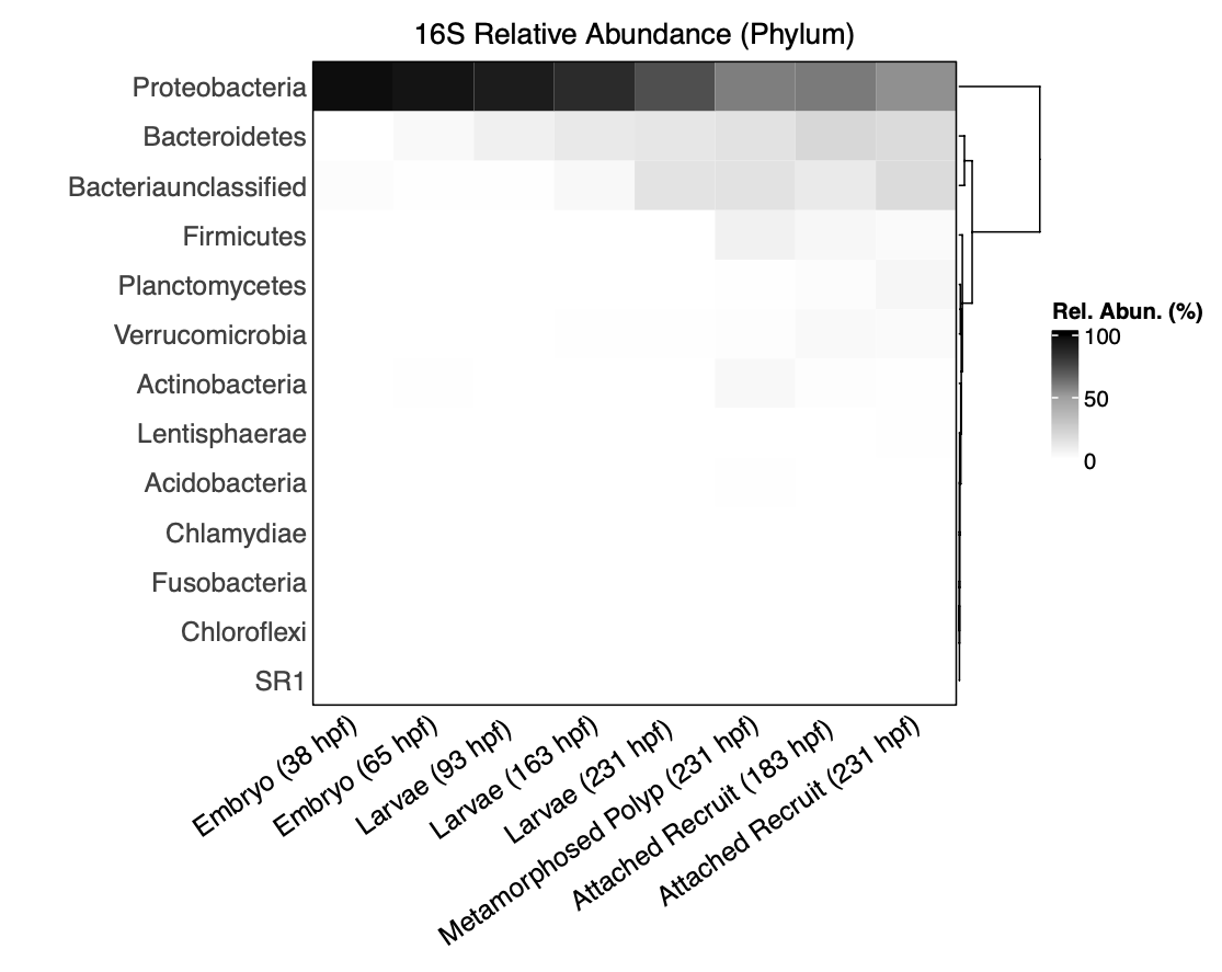
We see that samples are dominated by Proteobacteria. It appears that Bacteriodes and unclassified Bacteria increase in later life stages.

Then I vizualized relative abundance at the level of Genus:Family. Note that after filtering for taxa <1% relative abundance, we are left with 16 taxa.

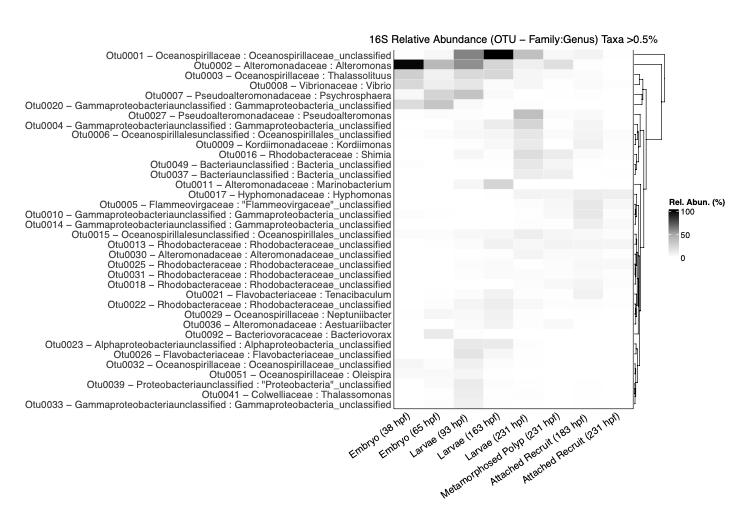
From this dataset, we can specifically look at comparisons of lifestages within the pre-183 hpf and comparison of lifestages within the time period after 183 hpf.

I noticed that in earlier lifestages there is a higher prevalence of Vibrio spp. There is also a peak of Oceanosprilliacaea (unclassified) in mid points of early life history. Alteromonas peaks in early stages of embryos. Pseudoalteromonas, Rhodobacteraceae, and Kordiimonadaceae are more prevalent in later time points.

Next Steps

The next steps will be to look at the taxa present in samples more closely and consult with collaborators on this data set.