


Mcapitata Larval Temperature Experiment Data Analysis
This post details analysis of survival, settlement, physiology, and environmental data for the 2021 Montipora capitata larval temperature project.
For more information on this project, refer to previous notebook posts and the GitHub repo.
Overview
This notebook post details the most recent data analysis for this project completed in February 2023. Data analyzed includes larval protein content, symbiont cell density, respirometry data (respiration and photosynthesis), carbohydrate content, survival, and settlement. Environmental analyses are also included in this post.
The final dataset for this project is stable isotope metabolomics, which is currently being processed at Rutgers University and results are pending.
Scripts and all data can be found on the GitHub repo for this project.
1. Environmental Data
We collected temperature data during this experiment every 10 minutes using Hobo loggers. I plotted this data over the course of the experiment.
Figure 1. Temperatures over the course of the experiment in high (red) and ambient (blue) treatments. Reproduction of M. capitata occured during the new moon and larvae were reared until the planua stage. I sampled initial samples (indicated by “*”) and then started temperature treatments (dotted line). Larvae were exposed to elevated (+2.5°C) or ambient temperatures over 3 days, after which they were sampled for physiology and metabolomics (indicated by “+”). Larvae were then moved into settlement chambers (solid line) to monitor settlement in high and ambient conditions.
| Period | High | Ambient |
|---|---|---|
| Embryo Rearing | 26.5 | 26.5 |
| Larval Exposure | 29.2 | 26.7 |
| Settlement | 29.2 | 27.2 |
2. Survival
I measured survival every 12 hours during the larval exposure period as the density of larvae (larvae per mL) in each tank (n=12 tanks, n=6 tanks per temperature). Survival is then plotted as the number of larvae per mL across the exposure period.
Figure 2. Larval survival at ambient (blue) and high (red) temperature treatments. Larval survival displayed as larval concentration (larvae per mL).
Survival was analyzed using a linear mixed effect model with tank as a random effect due to repeated measures. In all models, assumption of normal residuals and homogeneity of variance of residuals was assessed with qqPlots and Levene’s tests, respectively.
survmodel<-lmer(Larvae.per.mL~Treatment*Timepoint + (1|Tank:Treatment:Timepoint), data=survival)
anova(survmodel, type="II")
qqPlot(residuals(survmodel))
leveneTest(residuals(survmodel)~Treatment*Timepoint, data=survival)
As seen in the plot above, time was a significant driver of survival with approx. 25% decrease in survival on the last day of the experiment regardless of treatment. There was no effect of treatment on survival. Due to the rapid increase in mortality on the last day, we sampled for physiology and metabolomics at that point.
3. Settlement
After sampling, the remaining larvae were placed in settlement chambers to monitor settlement rate at the respective temperatures.
Figure 3. Larval settlement rates at ambient (blue) and high (red) temperature treatments. Settlement expressed as % settlement.
Settlement was analyzed using a linear mixed effect model with tank as a random effect due to repeated measures.
settlemodel<-lmer(Settled~Treatment*Date + (1|Tank:Treatment:Date), data=settle)
anova(settlemodel, type="II")
Settlement rates increased across the 5 day monitoring period to total approximately 10% at the end of the study. There was no difference in settlement due to treatment (p-values seen in Figure 3).
4. Respirometry
During the experimental sampling, I measured photosynthesis and respiration of larvae from each treatment to 27°C and 30°C in a reciprocal exposure design.
Figure 4. Respiration (A), Net Photosynthesis (B), Gross Photosynthesis (C), and P:R ratio (D) for larvae from ambient (blue) and high (red) treatments at 27°C and 30°C (x-axis). Metabolic rates normalized to per larva.
Metabolic rates were analyzed using an Analysis of Variance test (ANOVA) using the following structure:
model<-aov(rate~Treatment*Temperature, data=PRdata)
summary(model)
Respiration rates were not different by rearing treatment (ambient or high) or measurement temperature. There was also no effect of treatment or temperature on Gross Photosynthesis. Interestingly, There was an effect of rearing treatment on Net Photosynthesis (excess oxygen produced after accounting for oxygen consumption through respiration). Net photosynthesis was higher in larvae reared at high temperature (Figure 4) (p=0.035). Further, there was no significant difference in P:R ratio (as expected due to no difference in Respiration and Gross Photosynthesis values), but there was a trend for higher P:R in high treatment larvae (p=0.051).
Collectively, this data shows that M. capitata larvae may be metabolically resilient to shifts in temperature in our study and that our temperature treatments were not large enough or long enough to elicit a physiological response. The increase in Net Photosynthesis is interesting and aligns with our understanding that as temperature increases, metabolic rates increase due to enzymatic activity. It is possible that at elevated temperatures, Rubisco activity is increased in larvae, resulting in higher photosynthesis rates. We will explore this hypothesis with the metabolomic data when it becomes available. This has interesting implications for how larvae respond to moderate temperature stress and may point to increased thermal tolerance in the M. capitata population in Kaneohe Bay.
5. Physiology
In Spring 2021, I travelled to Rhode Island to process physiological samples, detailed in a previous notebook post. All physiological metrics were analyzed on the same larval pool (i.e., all metrics analyzed on each larval tube to allow for normalization).
All physiological data is presented in the following figure:
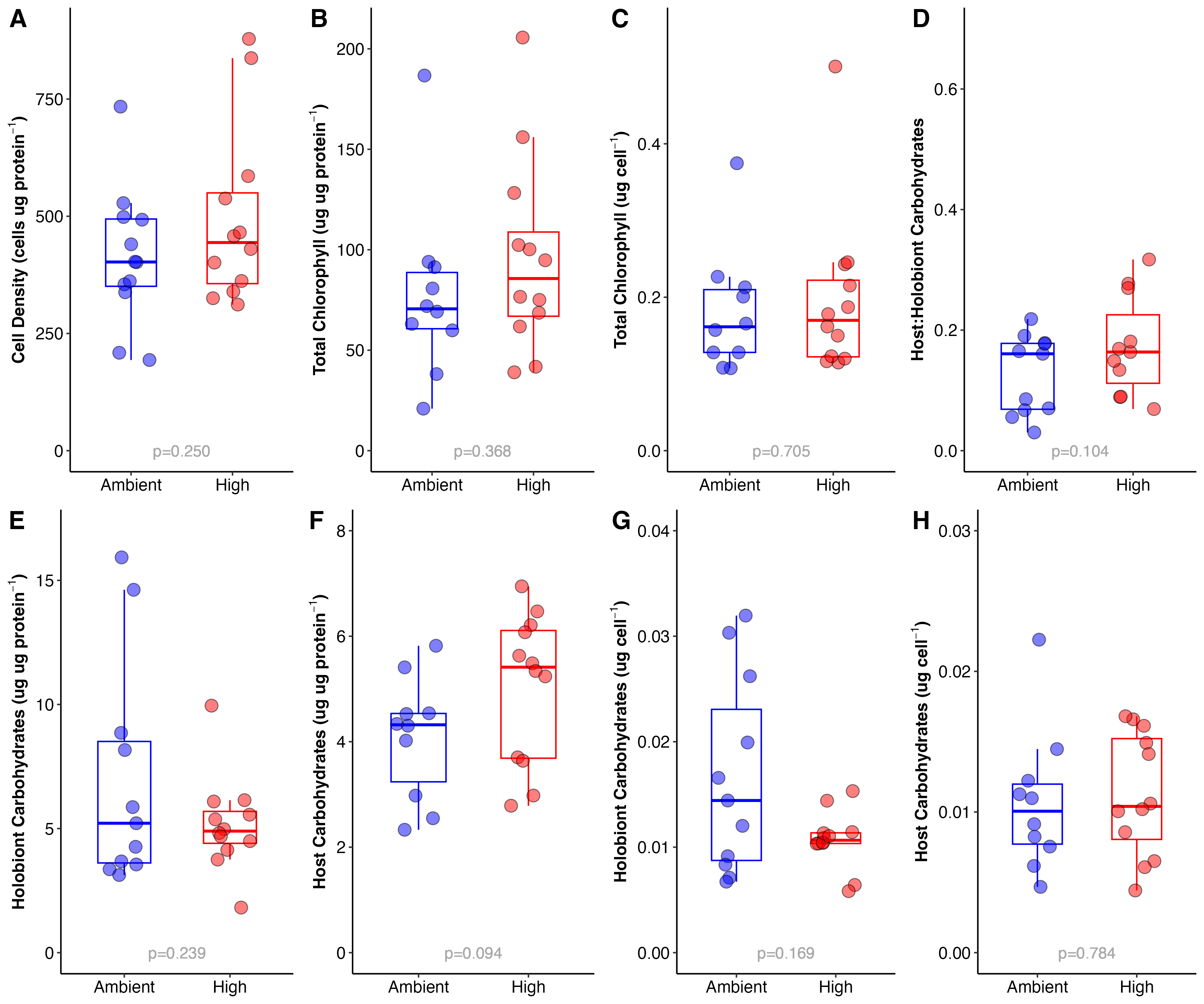
Figure 5. Physiological responses of larvae to ambient (blue) and high (red) thermal treatments. Responses include symbiont cell density (A), chlorophyll (B-C), and carbohydrate content (D-H). Note that metrics were normalized either to host protein or symbiont cell density (per cell).
Protein assays were conducted as a normalizing variable for these responses. Protein content was not analyzed independently. For protein and carbohydrate assays, we analyzed data in several runs and generated standard curves for each run. I then applied standard curve regressions to samples in a loop as in the example below for carbohydrates:
run_list<-c("1", "2", "3")

df_carbs = data.frame()

for (run in run_list) {

  #subset data
Standard <- carbs_data %>%
  filter(Sample.Type == "Standard")%>%
  filter(Run==run)

#generate standard curve equation
lmstandard <- lm (Concentration ~ abs.corr, data = Standard)
lmsummary <- summary(lmstandard)

#select samples
Samples <- carbs_data %>% #subsetting Samples
  filter(Sample.Type == "Sample")%>%
  filter(Run==run)

#calculate concentration
Samples$Concentration <- predict(lmstandard, newdata = Samples) #using model to get concentration

#add run column
Samples$Run<-run

#normalize to homogenate volume
#Accounting for dilution factor (1000/100) and normalizing to homogenate volume
#Multiply sample concentration (mg/mL) by total slurry volume (mL) and dilution factor (1000/v of sample, usually 100 mL)

Samples$Carb.mg <- (Samples$Concentration * (Samples$Resuspension_volume/1000) * (1000/Samples$Homo_vol))

#join dataframes
df <- data.frame(Samples)
df_carbs <- rbind(df_carbs,df)

}
This approach was very useful for applying independent standard curves to each run using a simple script in R.
Cell Density
Cell density was normalized to host protein and analyzed using an ANOVA.
sym_model<-aov(cells.ugprotein~Treatment, data=sym_model_data)
summary(sym_model)
There was no difference in cell density between treatments (Figure 5A).
Chlorophyll
We measured chlorophyll a and chlorophyll c2, normalized both to host protein and symbiont cell density in larvae from each treatment. I found that there was no difference in a and c2 by treatment.
Protein-normalized chlorophyll content:
chla_prot_model<-aov(chlA.ug.protein.ug~Treatment, data=df_chl)
summary(chla_prot_model)

            Df Sum Sq Mean Sq F value Pr(>F)
Treatment    1    513   513.1   0.925  0.348
Residuals   20  11090   554.5
chlc2_prot_model<-aov(chlC2.ug.protein.ug~Treatment, data=df_chl)
summary(chlc2_prot_model)

            Df Sum Sq Mean Sq F value Pr(>F)
Treatment    1    398   398.4   0.399  0.535
Residuals   20  19978   998.9
Cell-normalized chlorophyll content:
chla_cell_model<-aov(chlA.ug.cell~Treatment, data=df_chl)
summary(chla_cell_model)

            Df  Sum Sq   Mean Sq F value Pr(>F)
Treatment    1 0.00000 0.0000000       0  0.998
Residuals   20 0.01298 0.0006489
chlc2_cell_model<-aov(chlC2.ug.cell~Treatment, data=df_chl)
summary(chlc2_cell_model)

            Df  Sum Sq  Mean Sq F value Pr(>F)
Treatment    1 0.00129 0.001288   0.204  0.656
Residuals   20 0.12593 0.006296
Because the concentrations of both of these pigments were not different by treatment, I added them together to represent total chlorophyll content.
Total chlorophyll content:
I analyzed total chlorophyll content normalized to both protein and cell density (Figure 5BC).
chl.total_prot_model<-aov(total.chl.ug.protein.ug~Treatment, data=df_chl)
summary(chl.total_prot_model)

chl.total_cell_model<-aov(total.chl.ug.cell~Treatment, data=df_chl)
summary(chl.total_cell_model)
There was no difference in content by treatment (see Figure 5 for signifcance values).
Carbohydrates
Carbohydrate content was measured in both the host tissue and the holobiont (host + symbiont) tissue fractions. I calculated several metrics for carbohydrate content including host and holobiont carbohydrates normalized to both cell density and protein content and host:holobiont carbohydrate ratio. The ratio could indicate if there is a shift in carbohydrate allocation because a higher ratio would indicate an increase in carbohydrates in the host tissue relative to the holobiont as a whole.
Host:Holobiont ratios
Host:holobiont carbohydrate ratios are shown in Figure 5D and were not significantly different by treatment, but there was a trend for a higher ratio in the high temperature treatment. Ratios were analyzed using an ANOVA. I also ran non-parametric tests and got the same answer as the ANOVA analysis.
model<-aov(ratio~Treatment, data=carb_ratio)
summary(model)
The trend for a higher ratio for larvae from high temperature suggests that there may be more translocation of carbohydrates from the symbiont to the host. This would line up with data indicating photosynthesis rates are higher at elevated temperature. We will test this hypothesis with the metabolomic data when available. It is possible that M. capitata are metabolically resilient to this moderate temperature increase and that they could actually get more nutrition from symbionts that are fixing more carbon through photosynthesis.
Host carbohydrate content
Host carbohydrate content normalized to protein and cell density was analyzed and were not different by treatment (Figure 5FH). However, there was a trend for increased host carbohydrates normalized to proteins (p=0.099), but this trend was not seen when normalized to symbiont cell density.
model<-aov(Carb.prot~Treatment, data=model_data)
summary(model)

model<-aov(carbs.cell~Treatment, data=cells_data_model)
summary(model)
Holobiont carbohydrate content
Holobiont carbohydrate content normalized to protein and cell density was analyzed using an ANOVA. Interestingly, when normalized to protein, there was no difference in holobiont protein between treatments. But when normalized to cell density, there were significantly less carbohydrates in the high temperature larave at the holoboint level (p=0.046) and this was less variable (Figure 5EG). This indicates that there are less carbohydrates per symbiont cell in the holobiont tissues at high temperature. Because there was no difference in cell densities (Figure 5A), this is likely not driven by cell density and rather by total carbohydrate content. One possible explanation is that high temperature larvae are consuming carbohydrates at an elevated rate, although if this was the case we would expect elevated respiration rates. To understand what is underlying these differences, we need to examine the metabolomic data when it is availble.
model<-aov(Carb.prot~Treatment, data=model_data)
summary(model)

model<-aov(carbs.cell~Treatment, data=cells_data_model)
summary(model)
Larval Size
Finally, we imaged larvae preserved from each treatment to examine larval size calculated as volume of each individual larva at the end of the exposure period.
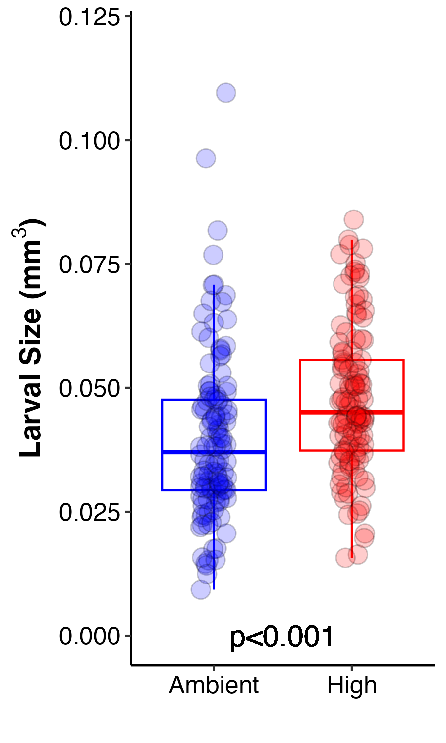
Figure 6. Larval size calculated as larval volume at ambient (blue) and high (red) temperature treatments.
Larval size was analyzed using an ANOVA.
model2<-aov(volume.mm3~treatment, data=model_data)
summary(model2)
Larvae from the high temperature treatment were significantly larger than those at ambient. The difference was small, but highly significant due to high sample size. This suggests that larvae had higher growth rates and/or had lower rates of consumption of lipid reserves therefore retaining a larger size. Larval size is generally associated with greater fitness and competency, including greater potential for dispersal. I hypothesize that larvae are larger due to increased photosynthesis and therefore translocation of nutritional compounds from the symbiont allowing the larvae to use energy reserves at reduced rates. This will be tested by examining the metabolomic data when available.