This post details continued analysis of metabolomics data for the 2020 M. capitata developmental time series with WGCNA.

WGCNA metabolomics analysis - part 2

All scripts and analyses can be found in my GitHub.

Kevin Wong further revised the WGCNA metabolomics pipeline with his scripts found here.

I conducted previous WGCNA analysis on metabolomics data detailed in the Part 1 post.

Today, I revised this script to build off of Kevin Wong’s approach. This simplifies the script and uses blockwiseModules rather than dynamicTreeCut to generate modules.

Revised WGCNA

This WGCNA analysis was based on scripts by both myself and Kevin Wong. This revised approaches uses Blockwise Modules to designate modules of metabolites. This script combines adjacency calculations and substantially shortens the script.

The pipeline workflow is as follows:

1. Data preparation
   • Load and format clean data
   • Data filtering: PoverA and genefilter
   • Outlier detection
2. Network construction and consensus module detection
   • Choosing a soft-thresholding power: Analysis of a network topology β
   • Identify modules using blockwiseModules
   • Relate modules to sample information
   • Relate modules to life stage
3. Plot module-trait associations
4. Plot mean eigengene values for each module
5. Pathway analysis

1. Data preparation

Data is loaded and we select some important parameters.

We need to select a pOverA value. This specifyies the minimum count for a proportion of samples for each metabolite. Here, we are using a pOverA of 0.07. This is because we have 46 samples with a minimum of n=2 samples per lifestage. Therefore, we will accept genes that are present in 2/46 = 0.04 of the samples because we expect different metabolites by life stage as demonstrated by PLSDA analysis as analyzed in other metabolomic analyses. We are further setting the minimum value of metabolites to 1 (median normalized), such that 4% of the samples must have a non-zero normalized metabolite presence in order for the metabolite to remain in the data set.

After data is loaded, we can proceed with network construction and consensus module detection.

2. Network construction

In this step, we construct a network and detect modules using the blockwiseModules function in the wgcna package.

First, we select a soft thresholding power. The soft thresholding power (β) is the number to which the co-expression similarity is raised to calculate adjacency. The function pickSoftThreshold performs a network topology analysis.

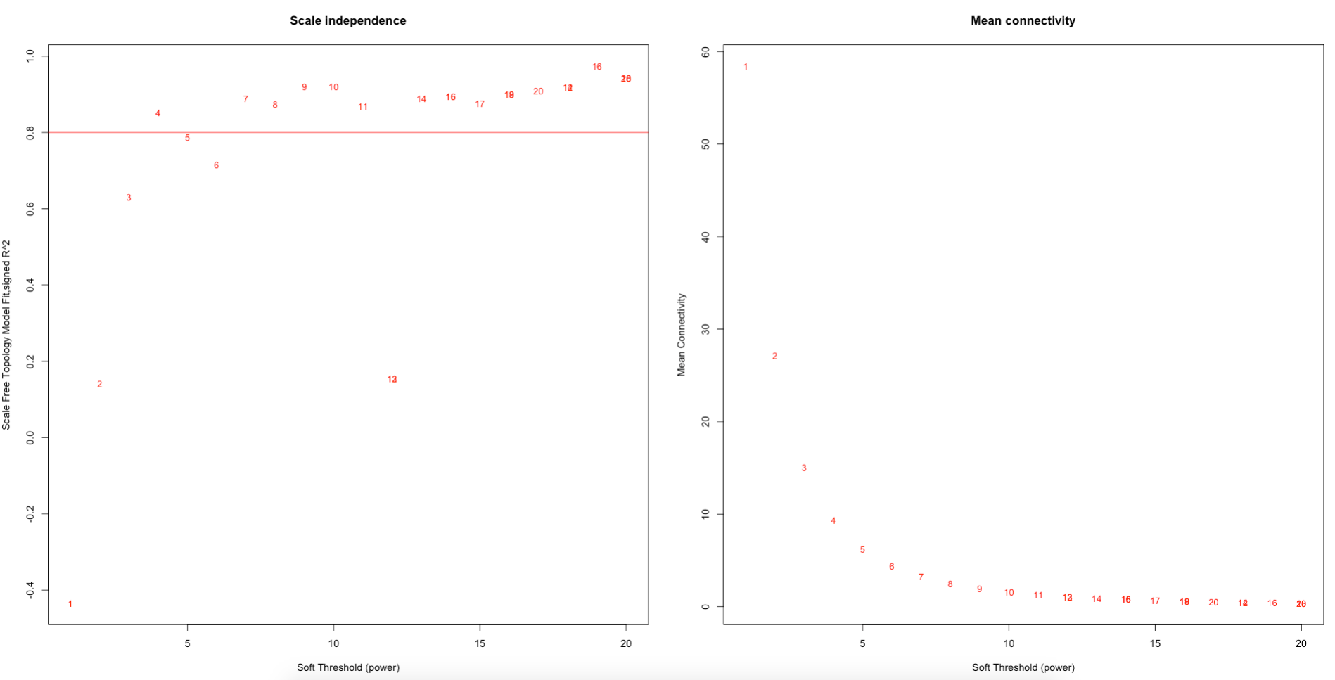
Here, we selected a threshold value of 7.

We then use blockwiseModules to construct network and identify modules.

The script looks like this:

picked_power = 7
temp_cor <- cor       
cor <- WGCNA::cor                                             # Force it to use WGCNA cor function (fix a namespace conflict issue)
netwk <- blockwiseModules(data_filt,                         # <= input here

                          # == Adjacency Function ==
                          power = picked_power,               # <= power here
                          networkType = "unsigned",

                          # == Tree and Block Options ==
                          deepSplit = 2,
                          pamRespectsDendro = F,
                          # detectCutHeight = 0.75,
                          minModuleSize = 5,                  #consider increasing or decreasing this
                          maxBlockSize = 4000,

                          # == Module Adjustments ==
                          reassignThreshold = 0,
                          mergeCutHeight = 0.25,

                          # == TOM == Archive the run results in TOM file (saves time) but it doesn't save a file
                          saveTOMs = F,
                          saveTOMFileBase = "ER",

                          # == Output Options
                          numericLabels = T,
                          verbose = 3)

cor <- temp_cor     # Return cor function to original namespace

# Identify labels as numbers 
mergedColors = netwk$colors
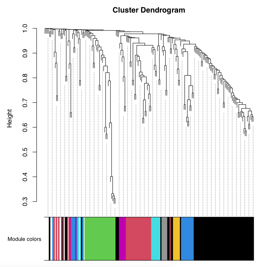
# Plot the dendrogram and the module colors underneath

pdf("Mcap2020/Figures/Metabolomics/WGCNA/blockwise_module_colors.pdf")
plotDendroAndColors(
  netwk$dendrograms[[1]],
  mergedColors[netwk$blockGenes[[1]]],
  "Module colors",
  dendroLabels = FALSE,
  hang = 0.03,
  addGuide = TRUE,
  guideHang = 0.05 )
dev.off()

The module dendrogram looks like this with colors indicating different modules:

We then load metadata and relate sample number to important metadata, including developmental time (hours post fertilization) and lifestage group (e.g., eggs, embryos).

3. Plotting module trait associations

Next we use complexHeatmap to plot the relationship between modules and traits. Here, the trait is the developmental time point, which is a binary variable with 0 or 1 for each stage category.

Our new heatmap looks like this:

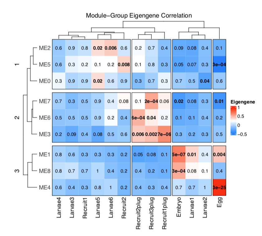
We can see that there are 3 “clusters” of modules with three modules each. These module clusters are associated with eggs and embryos (cluster 3), larvae and metamorphosed recruits (cluster 3), and attached recruits (cluster 2).

We can also plot the mean eigengene value (expression) of these clusters to see enrichment of these metabolite groups over development.

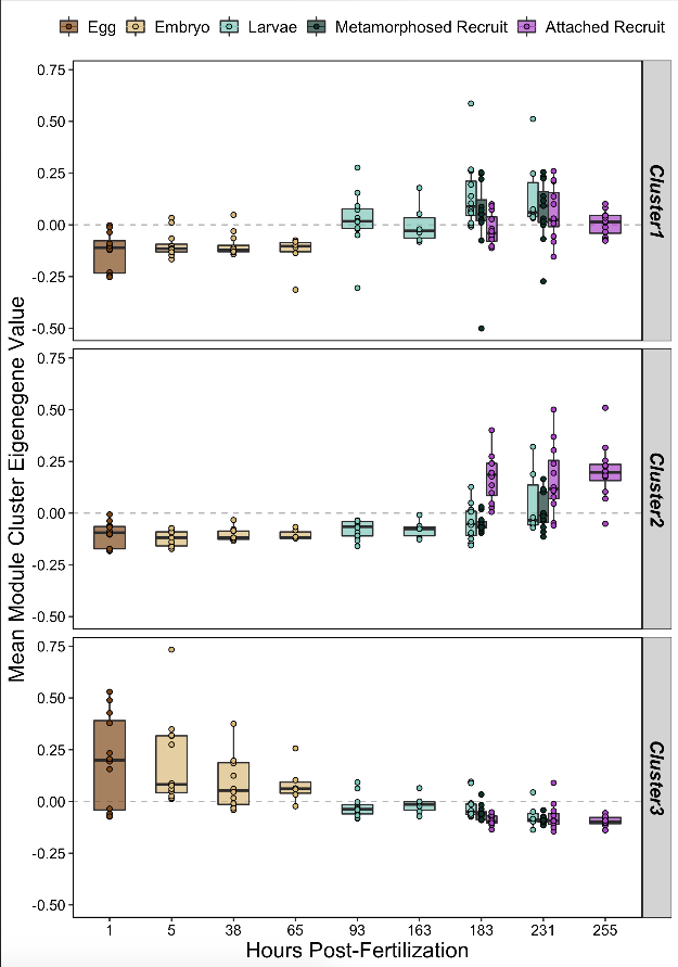
These clusters have clear differences in expression patterns over development.

Next, we will use metaboanalyst to look at enrichment and pathway analyses of the metabolites in these three module clusters.

Enrichment and Pathway Analyses

My goal for this portion of the analysis was to use the R version of Metaboanalyst through the MetaboAnalystR package. However, there are many difficulties with getting this package up and running. Here are a couple of the issues I had and the resolutions.

• Errors in package install: The package had issues with installation in R using devtools::install_github("xia-lab/MetaboAnalystR", build = TRUE, build_vignettes = FALSE). The errors came from dependencies not loading properly. I was able to see the packages that were required in an output error message and individually ensured that they were downloaded. Installation of MetaboAnalystR was then successful.
• Errors in the CrossReference function of metaboanalyst. This function reads in the reference database that your samples are matched to. I tried re installing curl, libcurl, xcode, and gfortran following error codes. However, this did not solve the problem. The problem remains that my computer has a permissions error preventing download that I was not able to resolve.

Therefore, rather than running in R code, I decided to run analyses in Metaboanalyst web interface. I will continue to trouble shoot this step to try to produce R code to run these steps.

Instead, I copied a list of metabolites in each module into MetaboAnalyst and conducted 1) Enrichment compound class and 2) Enrichment KEGG pathway analyses. This provides information on significantly enriched compound classes and KEGG pathways in each cluster, which we can relate to the lifestages correlated with these clusters.

Compound class results look like this:

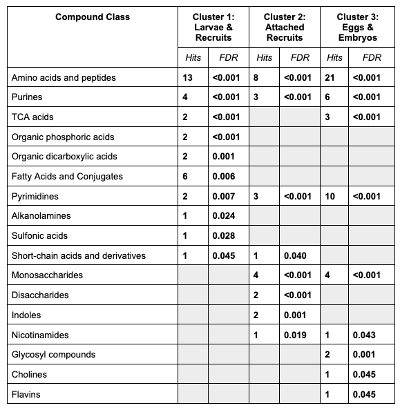
We see that each cluster has has unique compound classes. All clusters were enriched in amino acids and peptides.

KEGG pathway results look like this:

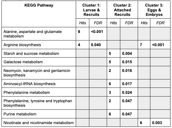
It is interesting to note that there are more pathways significantly enriched in attached recruits - particularly starch metabolim, a potential indicator of utilization of symbiotic nutrition.

We will continue to explore these data in our manuscript and this concludes the analysis of metabolite data!