


Revising E5 Time Series Multivariate Plasticity Analysis
This post details revisions to calculations for multivariate physiological plasticity analysis for the E5 Rules of Life project.
All code used in this post can be found in the E5 GitHub repository.
The original analysis and description of calculations can be found in this post.
Overview
The E5 physiological time series project includes data on coral and symbiont physiology in colonies of Acropora, Pocillopora, and Porites corals in Moorea, French Polynesia. Samples of individual colonies were collected at four timepoints in the year of 2020: Jan, Mar, Sep, and Nov.
For the physiological responses collected (e.g., biomass, symbiont density, calcification, protein, antioxidant capacity), we have analyzed to investigate the influence of species, site, and time on physiology. We have found that physiological response of corals is influenced by environmental variability both across space (site) and seasons (time point).
This can be visualized using trajectory principle component analyses, which visually show the movement in physiological trajectories of each species across space and time.

The next step in our analysis is to quantify the “movement” or physiological acclimatization in corals between species and sites. To do this, we conducted an analysis to quantify the differences in physiological profiles for each colony across time in multivariate space. This post detials our original analysis to do this and quanify physiological plasticity.
Revisions to Analysis
Previously, we utilized Euclidean distance in multivariate physiological profiles for each colony across time. I calculated the Euclidean distance between the PCA coordinates (using all PC’s) for each colony between Jan - Mar, Jan - Sept, and Jan - Nov.
Because these calculations were conducted from the change from the first time point to subsequent time points, we are missing some of the information on the total distance traveled (i.e., dispersion). To do this, I am going to calculate the euclidean distances for each colony as: Jan to Mar + Mar to Sept + Sept to Nov = total dispersion. This will provide a more accurate calculation of physiological plasticity across the time series.
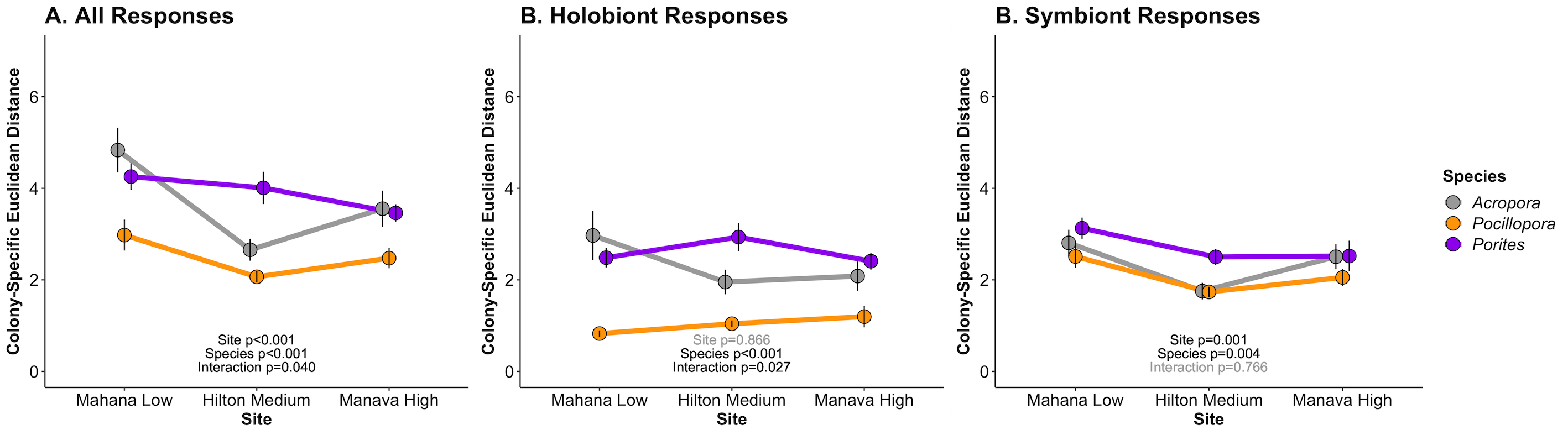
The previous analysis produced the following figure, which we will compare to at the end of this analysis.
Revising Calculations
See the previous notebook post for code for previous calculations as described above. In this analysis, I am using the same approach, but changing the equation for calculating the distances between time points for each colony.
All scripts in this post can be found in the E5 GitHub here.
First, I generated a dataframe that calculated the euclidian distance between all timepoints for each colony in a pairwise comparison.
data_all<-master%>%
  select(colony_id_corr, timepoint, species, site_code, Host_AFDW.mg.cm2, Sym_AFDW.mg.cm2, Ratio_AFDW.mg.cm2, prot_mg.mgafdw, cells.mgAFDW, cre.umol.mgafdw, Am, AQY, Rd, calc.umol.mgAFDW.hr, Total_Chl, Total_Chl_cell)%>%
  filter(Host_AFDW.mg.cm2>0)%>%
  filter(Sym_AFDW.mg.cm2>0)%>%
  filter(Ratio_AFDW.mg.cm2>0)%>%
  filter(Sym_AFDW.mg.cm2<20)%>%
  filter(prot_mg.mgafdw<1.5)%>% #remove outliers
  rename(Host_Biomass=Host_AFDW.mg.cm2, Symbiont_Biomass=Sym_AFDW.mg.cm2, S_H_Biomass_Ratio=Ratio_AFDW.mg.cm2, Host_Protein=prot_mg.mgafdw, Symbiont_Density=cells.mgAFDW, Antiox_Capacity=cre.umol.mgafdw, Calc=calc.umol.mgAFDW.hr) #select data of interest

head(data_all)

data_all<-data_all[complete.cases(data_all), ] #keep only complete cases

scaled_all<-prcomp(data_all[c(5:16)], scale=TRUE, center=TRUE) #scale and center data for pca analysis

all_info<-data_all[c(1:4)] #keep metadata

#generate a euclidean distance matrix between all samples (colony x time point)
all_data<-scaled_all%>%
  augment(all_info)%>%
  group_by(timepoint, site_code, species, colony_id_corr)%>%
  mutate(code=paste(timepoint, colony_id_corr))

all_data<-as.data.frame(all_data) #turn to data frame

row.names(all_data)<-all_data$code #rename rows

all_data<-all_data[6:17] #keep only data columns
head(all_data)

dist_all<-dist(all_data, diag = FALSE, upper = FALSE, method="euclidean") #calculate euclidian distance

dist_all <- melt(as.matrix(dist_all), varnames = c("row", "col")) #melt into data frame

head(dist_all) #view data
The data looked like this:
                 row                col    value
1 timepoint1 ACR-139 timepoint1 ACR-139 0.000000
2 timepoint1 ACR-140 timepoint1 ACR-139 1.326741
3 timepoint1 ACR-145 timepoint1 ACR-139 2.167381
4 timepoint1 ACR-150 timepoint1 ACR-139 3.161184
5 timepoint1 ACR-165 timepoint1 ACR-139 2.045959
6 timepoint1 ACR-173 timepoint1 ACR-139 1.217943
Second, I selected only the comparisons that we want to calculate (Jan-March, March-Sept, and Sept-Nov) for each colony and removed the duplicate reciprocal comparisons (Jan-March distance and March-Jan distance, which are the same).
I then generated rules to calculate distances. This was complicated because we were often missing data from 1-3 time points for some colonies. This meant that I needed to make rules for calculating distances. For example, if a colony was missing data from March, I wanted to calculate the distance from January to September instead. Because we are looking at the sum of all distances, I only kept colonies that we had at least 3 time points of information. This resulted in 36 colonies out of 123 without plasticity calculations.
The code for these rules is below:
mutate(sum_1=rowSums(.[ , c("T1_T2", "T2_T3", "T3_T4")]))%>% #add all values for corals with all four timepoints recorded by summing T1-T2, T2-T3 and T3-T4
  mutate(sum_2=case_when(is.na(T1_T2) ~ rowSums(.[ , c("T1_T3", "T3_T4")])))%>% #If T2 is missing, instead sum T1-T3 and T3-T4
  mutate(sum_3=case_when(is.na(T1_T4) ~ rowSums(.[ , c("T1_T2", "T2_T3")])))%>% #If T4 is missing, instead sum T1-T2 and T2-T3
 mutate(sum_4=case_when(is.na(T1_T3) ~ rowSums(.[ , c("T1_T2", "T2_T4")])))%>% #If T3 is missing, instead sum T1-T2 and T2-T4
  mutate(sum_5=case_when(is.na(T1_T2) & is.na(T1_T3) & is.na(T1_T4) ~ rowSums(.[ , c("T2_T3", "T3_T4")])))%>% #If T1 is missing, instead sum T2-T3 and T3-T4
The full code for calculations and data manipulation are below here:
#calculate distances between subsequent time points (T1-T2, T2-T3, T3-T4) and sum them together

dist_all_calc<-dist_all%>%
  separate(row, into=c("Timepoint1", "Colony1"), sep=" ")%>%
  separate(col, into=c("Timepoint2", "Colony2"), sep=" ")%>%
  filter(value>0.0)%>% #remove distances between the same points
  mutate(condition=if_else(Colony1==Colony2, "TRUE", "FALSE"))%>%
  filter(condition=="TRUE")%>% #keep within colony comparisons
  arrange(Colony1, Timepoint1, Timepoint2)%>% #arrange by time points
  select(Timepoint1, Timepoint2, Colony1, value)%>%
  mutate(comparison=paste(Timepoint1, "-", Timepoint2))%>% #add a comparison column
  filter(!duplicated(paste(Colony1, value)))%>% #remove duplicated/reciprocal timepoint matches (e.g. timepoint1-timepoint2 and timepoint2-timepoint1)
  select(!Timepoint1)%>% #remove unneeded comments
  select(!Timepoint2)%>% #remove unneeded comments
  pivot_wider(names_from = comparison, values_from = value, id_cols=Colony1)%>% #move to wide format
  rename("T1_T2"="timepoint1 - timepoint2", #rename columns
         "T2_T3"="timepoint2 - timepoint3",
         "T3-T4"="timepoint3 - timepoint4",
         "T1_T3"="timepoint1 - timepoint3",
         "T1_T4"="timepoint1 - timepoint4",
         "T3_T4"="timepoint3 - timepoint4",
         "T2_T4"="timepoint2 - timepoint4")%>%
  mutate(sum_1=rowSums(.[ , c("T1_T2", "T2_T3", "T3_T4")]))%>% #add all values for corals with all four timepoints recorded by summing T1-T2, T2-T3 and T3-T4
  mutate(sum_2=case_when(is.na(T1_T2) ~ rowSums(.[ , c("T1_T3", "T3_T4")])))%>% #If T2 is missing, instead sum T1-T3 and T3-T4
  mutate(sum_3=case_when(is.na(T1_T4) ~ rowSums(.[ , c("T1_T2", "T2_T3")])))%>% #If T4 is missing, instead sum T1-T2 and T2-T3
 mutate(sum_4=case_when(is.na(T1_T3) ~ rowSums(.[ , c("T1_T2", "T2_T4")])))%>% #If T3 is missing, instead sum T1-T2 and T2-T4
  mutate(sum_5=case_when(is.na(T1_T2) & is.na(T1_T3) & is.na(T1_T4) ~ rowSums(.[ , c("T2_T3", "T3_T4")])))%>% #If T1 is missing, instead sum T2-T3 and T3-T4
  mutate(colony_dispersion=coalesce(sum_1, sum_2, sum_3, sum_4, sum_5))%>% #coalesce rows to remove na's and keep all summed values in one column
  select(Colony1, colony_dispersion) #keep colony ID and dispersion values

dist_all_calc$site_code<-master$site_code[match(dist_all_calc$Colony1, master$colony_id_corr)] #add in site code information
dist_all_calc$species<-master$species[match(dist_all_calc$Colony1, master$colony_id_corr)] #add in species information
This produced data that looked like this:
  Colony1 colony_dispersion site_code   species
  <chr>               <dbl> <fct>       <chr>
1 ACR-139             10.0  Manava High Acropora
2 ACR-140             12.0  Manava High Acropora
3 ACR-145              8.95 Manava High Acropora
4 ACR-150             12.0  Manava High Acropora
5 ACR-173              6.28 Manava High Acropora
6 ACR-175              6.66 Manava High Acropora
Where colony_dispersion is the metric of interest to calculate plasticity.
This calculation process was repeated for Holobiont (all metrics), Host, and Symbiont metrics.
Plotting
I generated plots for these plasticity values at the Holobiont, Host, and Symbiont levels and displayed anova analyses on the effects of site and species on these values.
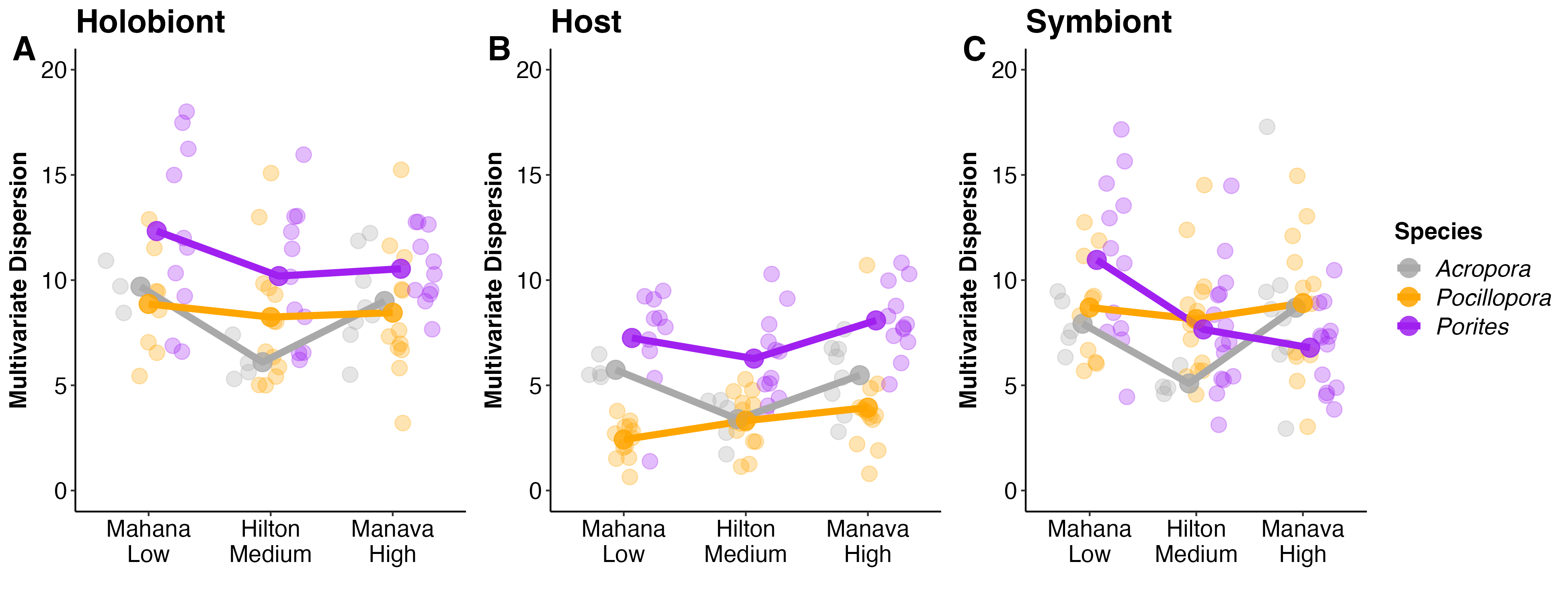
This figure shows multivariate dispersion, our metric of plasticity, on the y-axis across site and species. Each point is an individual colony with the group mean displayed in the dark lines and points. There are some interesting take aways from this analysis.
- Holobiont physiological plasticity was significantly different by species. Pocillopora had the lowest plasticity levels across site with Acropora and Porites more equal. There was a trend for reduced plasticity in Acropora at Hilton, but the site x species interaction was not significant.
- Host physiology was different by species as expected with lowest values in Pocillopora. The site x species interaction was significant. This is driven by higher plasticity in Acropora than Porites at Mahana, but lower in Acropora at Hilton. Plasiticty for each species was dependent on site.
- For both holobiont and host physiology, site was not significant, but there was a non-significant trend for variation by site.
- Symbiont physiology, interestingly, was not different by species or site. This suggests that holobiont plasticity was driven more by the host than the symbiont.
This interpretation differs from the previous version, where host and symbiont plasticity were significantly influenced by site and species.